Calculate shortest path(s) and/or distance(s) over a surface between origin and destination coordinates
Source:R/lcps.R
lcp_over_surface.RdThis function computes the shortest path(s) and/or distance(s) over a surface between origin and destination coordinates. To implement this function, origin and destination coordinates need to be specified as matrices and the surface over which movement occurs should be supplied as a raster. Since determining shortest paths can be computationally and memory-intensive, the surface can be reduced in size and/or resolution before these are computed, by (a) cropping the surface within user-defined extents; (b) focusing on a buffer zone along a Euclidean transect connecting origin and destination coordinates; (c) aggregating the surface to reduce the resolution; and/or (d) masking out areas over which movement is impossible (e.g., land for marine animals). Then, the function computes distances between connected cells, given (a) the planar distances between connected cells and (b) their difference in elevation. These distances are taken as a measure of `cost'. For each pair of origin and destination coordinates, or for all combinations of coordinates, these distances are used to compute the least-cost (i.e., shortest) path and/or the distance of this path, using functions in the cppRouting or gdistance package. The function returns the shortest path(s) and/or their distance(s) (m) along with a plot and a list of objects involved in the calculations.
lcp_over_surface(
  origin,
  destination,
  surface,
  crop = NULL,
  buffer = NULL,
  aggregate = NULL,
  mask = NULL,
  mask_inside = TRUE,
  plot = TRUE,
  goal = 1,
  combination = "pair",
  method = "cppRouting",
  cppRouting_algorithm = "bi",
  cl = NULL,
  varlist = NULL,
  use_all_cores = FALSE,
  check = TRUE,
  verbose = TRUE
)
Arguments
- origin
A matrix which defines the coordinates (x, y) of the starting location(s). Coordinates should lie on a plane (i.e., Universal Transverse Mercator projection).
- destination
A matrix which defines the coordinates (x, y) of the finishing location(s). Coordinates should lie on a plane (i.e., Universal Transverse Mercator projection).
- surface
A
rasterover which the object (e.g., individual) must move fromorigintodestination. Thesurfacemust be planar (i.e., Universal Transverse Mercator projection) with units of metres in x, y and z directions (m). Thesurface'sresolutionis taken to define the distance between horizontally and vertically connected cells and must be the same in both x and y directions (forsurface's with unequal horizontal resolution,resamplecan be used to equalise resolution: see Examples). Any cells with NA values (e.g., due to missing data) are treated as `impossible' to move though by the algorithm. In this case, thesurfacemight need to be pre-processed so that NAs are replaced/removed before implementing the function, depending on their source.- crop
(optional) An
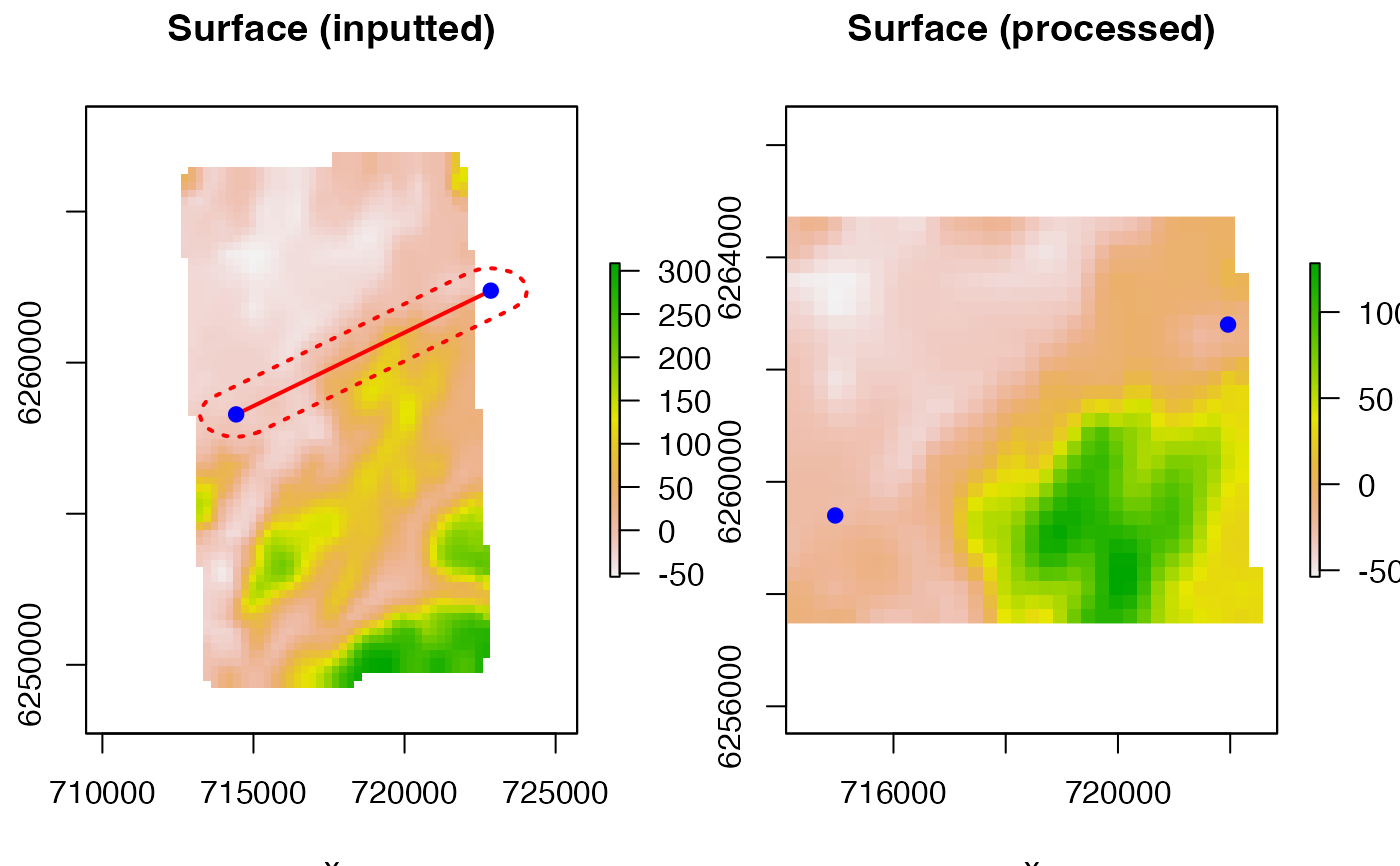
extentobject that is used tocropthe extent of thesurface, before the least-cost algorithms are implemented. This may be useful for large rasters to reduce memory requirements/computation time.- buffer
(optional) A named list of arguments, passed to
gBuffer(e.g.buffer = list(width = 1000)) (m) that is used to define a buffer around a Euclidean transect connecting theoriginanddestination. (This option can only be implemented for a singleoriginanddestinationpair.) Thesurfaceis then cropped to the extent of this buffer before the least-cost algorithms are implemented. This may be useful for large rasters to reduce memory requirements and/or computation time.- aggregate
(optional) A named list of arguments, passed to
aggregate, to aggregate raster cells before the least-cost algorithms are implemented. This may be useful for large rasters to reduce memory requirements and/or computation time.- mask
(optional) A Raster or Spatial
maskthat is used to prevent movement over `impossible' areas on thesurface. This must also lie on a planar surface (i.e., Universal Transverse Mercator projection). For example, for marine animals,maskmight be aSpatialPolygonsDataFramewhich defines the coastline. The effect of themaskdepends onmask_inside(see below).- mask_inside
A logical input that defines whether or not to mask the
surfaceinside (TRUE) or outside (FALSE) of themask(seemask_io).- plot
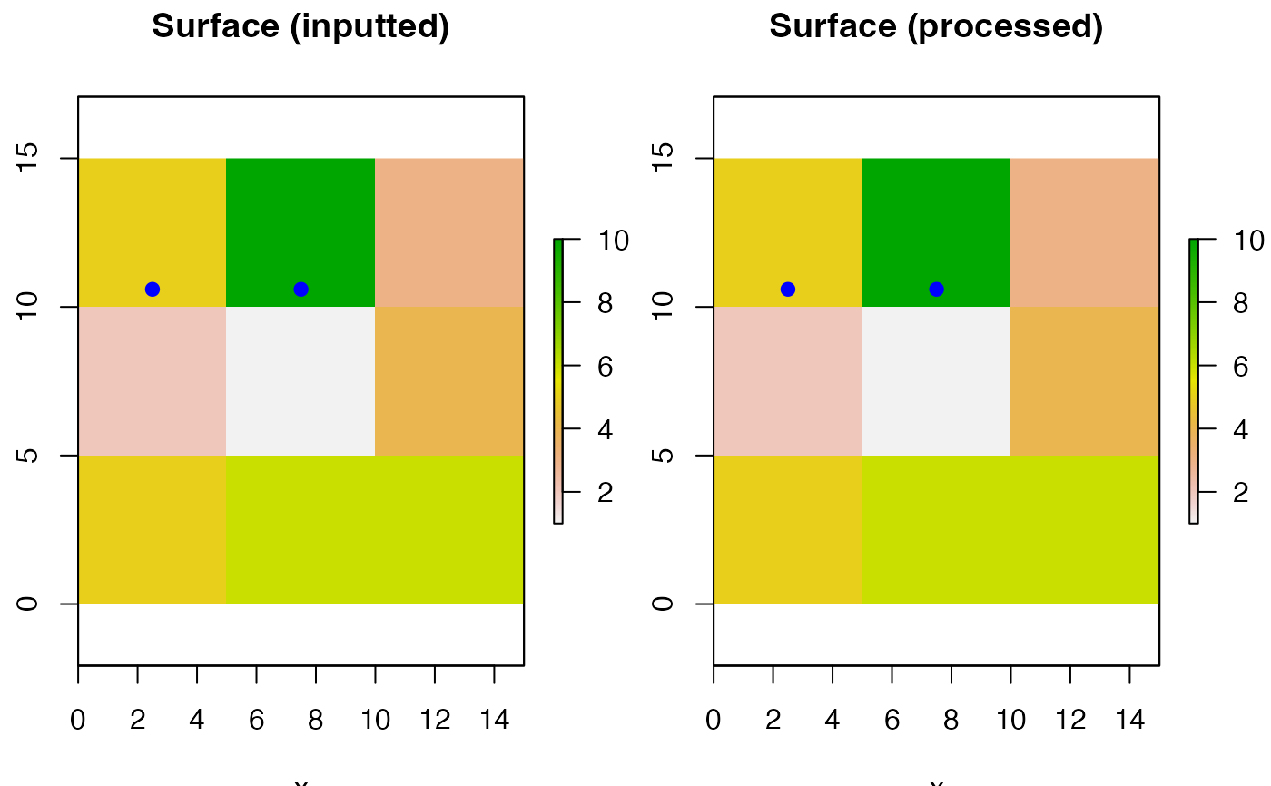
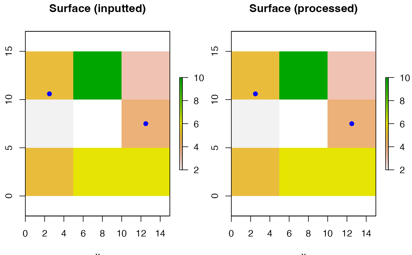
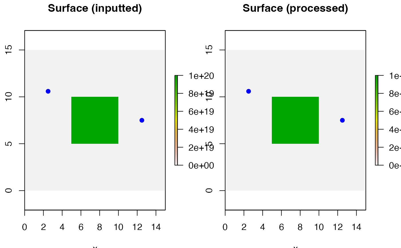
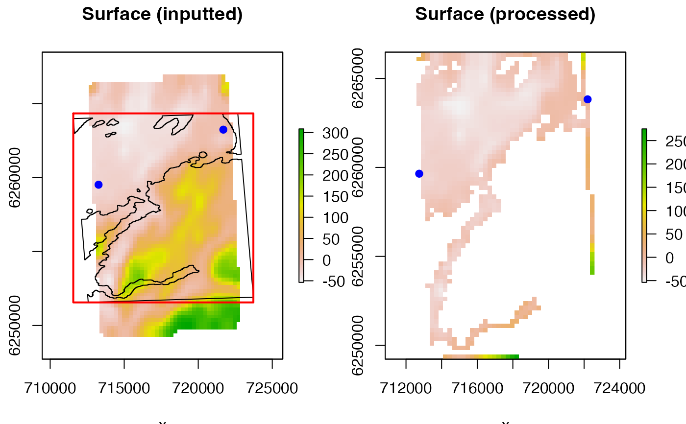
A logical input that defines whether or not to plot the inputted and processed surfaces. If
TRUE, the inputted and processed plots are produced side-by-side. For the inputted surface, themaskand the region selected (viacropand/orbuffer) are shown along with theoriginanddestination. For the processed surface, the surface and theoriginanddestinationare shown, along with the shortest path(s) (if and once computed: seegoal). This is useful for checking that anysurfaceprocessing steps have been applied correctly and theoriginanddestinationare positioned correctly on thesurface.- goal
An integer that defines the output of the function:
goal = 1computes shortest distances,goal = 2computes shortest paths andgoal = 3computes both shortest paths and the corresponding distances. Note thatgoal = 3results in least-cost algorithms being implemented twice, which will be inefficient for large problems; in this case, usegoal = 2to compute shortest paths and then calculate their distance using outputs returned by the function (see Value).- combination
A character string (
"pair"or"matrix") that defines whether or not to compute shortest distances/paths for (a) each sequentialoriginanddestinationpair of coordinates (combination = "pair") or (b) all combinations oforiginanddestinationcoordinates (combination = "matrix"). This argument is only applicable if there is more than oneoriginanddestination. Forcombination = "pair", the number oforiginanddestinationcoordinates needs to be the same, since eachoriginis matched with eachdestination.- method
A character string (
"cppRouting"or"gdistance") that defines the method used to compute the shortest distances between theoriginand thedestination."cppRouting"is the defaultmethod. Under this option, functions in thecppRoutingpackage are used to compute the shortest paths (get_path_pairorget_multi_pathsfor each pair of coordinates or for all combinations of coordinates, respectively) and/or distances (get_distance_pairorget_distance_matrix). This package implements functions written in C++ and massively outperforms the othermethod = "gdistance"for large problems. Otherwise, ifmethod = "gdistance", functions in thegdistanceare called iteratively to compute shortest paths (viashortestPath) or distances (viacostDistance).- cppRouting_algorithm
A character string that defines the algorithm used to compute shortest paths or distances. This is only applicable if
method = "cppRouting":method = "gdistance"implements Dijkstra's algorithm only. For shortest paths or their distances between pairs of coordinates, the options are"Dijkstra","bi","A*"or"NBA"for the uni-directional Dijkstra, bi-directional Dijkstra, A star unidirectional search or new bi-directional A star algorithms respectively (seeget_path_pairorget_distance_pair). For shortest paths between all combinations of coordinates,cppRouting_algorithmis ignored and the Dijkstra algorithm is implemented recursively. For shortest distances between all combinations of coordinates, the options are"phast"or"mch"(seeget_distance_matrix).- use_all_cores, cl, varlist
Parallelisation options for
method = "cppRouting"(use_all_cores) ormethod = "gdistance"(clandvarlist) respectively. Ifmethod = "cppRouting", parallelisation is implemented viause_all_coresfor computing shortest distances only (not computing shortest paths).use_all_coresis a logical input that defines whether or not to use all cores for computing shortest distance(s). Ifmethod = "gdistance", parallelisation is implemented viaclandvarlistfor both shortest paths and distances function calls.clis (a) a cluster object frommakeClusteror (b) an integer that defines the number of child processes.varlistis a character vector of variables for export (seecl_export). Exported variables must be located in the global environment. If a cluster is supplied, the connection to the cluster is closed within the function (seecl_stop). For further information, seecl_lapplyandflapper-tips-parallel.- check
A logical input that defines whether or not to check function inputs. If
TRUE, internal checks are implemented to check user-inputs and whether or not inputted coordinates are in appropriate places on the processedsurface(for instance, to ensure inputted coordinates do not lie over masked areas). This helps to prevent intractable error messages. IfFALSE, these checks are not implemented, so function progress may be faster initially (especially for largeorigin/destinationcoordinate matrices).- verbose
A logical input that defines whether or not to print messages to the console to monitor function progress. This is especially useful with a large
surfacesince the algorithms are computationally intensive.
Value
A named list
The function returns a named list. The most important element(s) of this list are `path_lcp' and/or `dist_lcp', the shortest path(s) and/or distance(s) (m) between origin and destination coordinate pairs/combinations. `path_lcp' is returned if goal = 2 or goal = 3 and `dist_lcp' is returned if goal = 1 or goal = 3. `path_lcp' contains (a) a dataframe with the cells comprising each path (`cells'), (b) a named list containing a SpatialLines object for each path (`SpatialLines') and (c) a named list of matrices of the coordinates of each path (`coordinates'). `dist_lcp' is a (a) numeric vector or (b) matrix with the distances (m) between each pair or combination of coordinates respectively. If `dist_lcp' is computed, `dist_euclid', the Euclidean distances (m) between the origin and destination, is also returned for comparison.
Common elements
Other elements of the list record important outputs at sequential stages of the algorithm's progression. These include the following elements: `args', a named list of user inputs; `time', a dataframe that defines the times of sequential stages in the algorithm's progression; `surface', the surface over which shortest distances are computed (this may differ from the inputted surface if any of the processing options, such as crop, have been implemented); `surface_param', a named list that defines the cell IDs, the number of rows, the number of columns, the coordinates of the implemented surface and the cell IDs of the origin and destination nodes; `cost', a named list of arguments that defines the distances (m) between connected cells under a rook's or bishop's movement (`dist_rook' and `dist_bishop'), the planar and vertical distances between connected cells (`dist_planar' and `dist_vertical') and the total distance between connected cells (`dist_total'); and `cppRouting_param' or `gdistance_param', a named list of arguments used to compute shortest paths/distances via cppRouting or gdistance (see below).
Method-specific elements
If method = "cppRouting", the `cppRouting_param' list contains a named list of arguments passed to makegraph (`makegraph_param') as well as get_path_pair (`get_path_pair_param') or get_multi_paths (`get_multi_paths_param') and/or get_distance_pair (`get_distance_pair_param') or get_distance_matrix (`get_distance_matrix_param'), depending on whether or not shortest paths and/or distances have been computed (see goal) and whether or not shortest paths/distances have been computed for each pair of coordinates or all combinations of coordinates. If method = "gdistance", this list contains a named list of arguments passed iteratively, for each pair/combination of coordinates, to shortestPath (`shortestPath_param') or costDistance (`costDistance_param'). This includes an object of class TransitionLayer (see Transition-classes), in which the transitionMatrix slot contains a (sparse) matrix that defines the ease of moving between connected cells (the reciprocal of the `dist_total' matrix).
Details
Methods
This function was motivated by the need to determine the shortest paths and their distances between points for benthic animals, which must move over the seabed to navigate from A to B. For these animals, especially in areas with heterogeneous bathymetric landscapes and/or coastline, the shortest path that an individual must travel to move from A and B may differ substantially from the Euclidean path that is often used as a proxy for distance in biological studies. However, this function can still be used in situations where the surface over which an individual must move is irrelevant (e.g., for a pelagic animal), by supplying a flat surface; then shortest paths/distances simply depend on the planar distances between locations and any barriers (e.g., the coastline). (However, this process will be somewhat inefficient.)
The function conceptualises an object moving across a landscape as a queen on a chessboard which can move, in eight directions around its current position, across this surface. Given the potentially large number of possible paths between an origin and destination, the surface may be reduced in extent or size before the game begins. To determine shortest path/distance over the surface between each origin and destination pair/combination, the function first considers the distance that an object must travel between pairs of connected cells. This depends on the planar distances between cells and their differences in elevation. Planar distances (\(d_p\), m) depend on the movement type: under a rook's movement (i.e., horizontally or vertically), the distance (\(d_{p,r}\)) between connected cells is extracted from the raster's resolution (which is assumed to be identical in the x and y directions); under a bishop's movement (i.e., diagonally), the distance between connected cells \(d_{p,b}\) is given by Pythagoras' Theorem: \(d_{p,b} = \sqrt{(d_{p, r}^2 + d_{p, r}^2)}\). Vertical distances (\(d_v\), m) are simply the differences in height between cells. The total distance (\(d_t\)) between any two connected cells is a combination of these distances given by Pythagoras' Theorem: \(d_t = \sqrt{(d_p^2 + d_v^2)}\). These distances are taken to define the `cost' of movement between connected cells. Thus, `costs' are symmetric (i.e., the cost of moving from A to B equals the cost of moving from B to A).
This cost surface is then used to compute the shortest path and/or distance of the shortest path between each origin and destination pair/combination using functions in the cppRouting or gdistance package. The functions implemented depend on the goal (i.e., whether the aim is to compute shortest paths, shortest distances or both) and, if there is more than one origin/destination, the combination type (i.e., whether to compute shortest paths/distances for each sequential pair of coordinates or all possible combinations of coordinates).
Warnings
The function returns a warning produced by transition which is implemented to facilitate the definition of the cost surface, before shortest paths/distances are computed by either method: `In .TfromR(x, transitionFunction, directions, symm) : transition function gives negative values'. This warning arises because the height differences between connecting cells can be negative. It can be safely ignored.
Examples
#### Example types
# Shortest distances between a single origin and a single destination
# Shortest paths between a single origin and a single destination
# Shortest distances/paths between origin/destination pairs
# Shortest distances/paths between all origin/destination combinations
#### Simulate a hypothetical landscape
# Define a miniature, blank landscape with appropriate dimensions
proj_utm <- sp::CRS(SRS_string = "EPSG:32629")
r <- raster::raster(
nrows = 3, ncols = 3,
crs = proj_utm,
resolution = c(5, 5),
ext = raster::extent(0, 15, 0, 15)
)
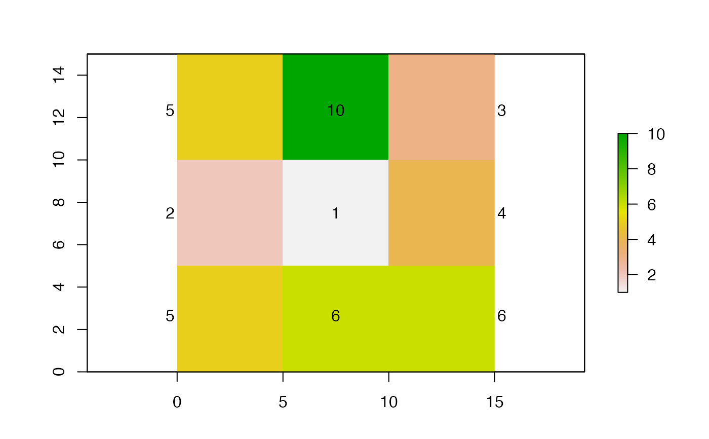
# Define a matrix of hypothetical values for the landscape
mat <- matrix(c(
5, 10, 3,
2, 1, 4,
5, 6, 6
), ncol = 3, nrow = 3, byrow = TRUE)
r[] <- mat
# Visualise simulated landscape
raster::plot(r)
raster::text(r)
 # Extract coordinates of cells
rxy <- raster::coordinates(r)
############################################################################
#### Shortest distances between a single origin and a single destination
#### Example (1): Find the distance between a single origin and destination
# ... using the "cppRouting" method:
out1 <- lcp_over_surface(
origin = rxy[1, , drop = FALSE],
destination = rxy[2, , drop = FALSE],
surface = r
)
#> flapper::lcp_over_surface() called (@ 2023-08-29 15:43:57)...
#> ... Checking user inputs...
#> ... Defining cost matrix...
#> Warning: transition function gives negative values
#> ... Calculating Euclidean distance(s)...
#> ... Using method = 'cppRouting'...
#> ... ... Defining nodes, edges and costs to make graph...
#> ... ... Constructing graph object...
#> ... ... Implementing bi algorithm to compute least-cost distance(s)...
#> ... flapper::lcp_over_surface() call completed (@ 2023-08-29 15:43:57) after ~0 minutes.
# Extract shortest distance
out1$dist_lcp
#> [1] 7.071068
#### Example (1) continued: An explanation of function outputs
# The function returns a list:
# The 'args' element simply contains all inputted arguments
out1$args
#> $origin
#> x y
#> [1,] 2.5 12.5
#>
#> $destination
#> x y
#> [1,] 7.5 12.5
#>
#> $surface
#> class : RasterLayer
#> dimensions : 3, 3, 9 (nrow, ncol, ncell)
#> resolution : 5, 5 (x, y)
#> extent : 0, 15, 0, 15 (xmin, xmax, ymin, ymax)
#> crs : +proj=utm +zone=29 +datum=WGS84 +units=m +no_defs
#> source : memory
#> names : layer
#> values : 1, 10 (min, max)
#>
#>
#> $crop
#> NULL
#>
#> $buffer
#> NULL
#>
#> $aggregate
#> NULL
#>
#> $mask
#> NULL
#>
#> $mask_inside
#> [1] TRUE
#>
#> $plot
#> [1] TRUE
#>
#> $goal
#> [1] 1
#>
#> $combination
#> [1] "pair"
#>
#> $method
#> [1] "cppRouting"
#>
#> $cppRouting_algorithm
#> [1] "bi"
#>
#> $cl
#> NULL
#>
#> $varlist
#> NULL
#>
#> $use_all_cores
#> [1] FALSE
#>
#> $check
#> [1] TRUE
#>
#> $verbose
#> [1] TRUE
#>
# The 'surface' element contains the surface used to compute shortest distances
# ... This may differ from $args$surface if cropped, buffered etc.
out1$surface
#> class : RasterLayer
#> dimensions : 3, 3, 9 (nrow, ncol, ncell)
#> resolution : 5, 5 (x, y)
#> extent : 0, 15, 0, 15 (xmin, xmax, ymin, ymax)
#> crs : +proj=utm +zone=29 +datum=WGS84 +units=m +no_defs
#> source : memory
#> names : layer
#> values : 1, 10 (min, max)
#>
# The 'surface_param' element contains the cell IDs, number of rows, cells and coordinates
# ... of this surface
out1$surface_param
#> $cells
#> [1] 1 2 3 4 5 6 7 8 9
#>
#> $nrow
#> [1] 3
#>
#> $ncol
#> [1] 3
#>
#> $coordinates
#> x y
#> [1,] 2.5 12.5
#> [2,] 7.5 12.5
#> [3,] 12.5 12.5
#> [4,] 2.5 7.5
#> [5,] 7.5 7.5
#> [6,] 12.5 7.5
#> [7,] 2.5 2.5
#> [8,] 7.5 2.5
#> [9,] 12.5 2.5
#>
#> $origin_cell
#> [1] 1
#>
#> $destination_cell
#> [1] 2
#>
# The 'cost' element is a list of objects that define the cost matrix:
# ... 'dist_rook' and 'dist_bishop' are matrices which define the distance of planar
# ... ... movement from one cell to any other cell under a rook's or bishop's movement.
# ... ... For example, the planar distance of moving from cell 1 to cell 2 to is 5 m:
out1$cost$dist_rook
#> 9 x 9 sparse Matrix of class "dsCMatrix"
#>
#> [1,] . 5 . 5 . . . . .
#> [2,] 5 . 5 . 5 . . . .
#> [3,] . 5 . . . 5 . . .
#> [4,] 5 . . . 5 . 5 . .
#> [5,] . 5 . 5 . 5 . 5 .
#> [6,] . . 5 . 5 . . . 5
#> [7,] . . . 5 . . . 5 .
#> [8,] . . . . 5 . 5 . 5
#> [9,] . . . . . 5 . 5 .
out1$cost$dist_bishop
#> 9 x 9 sparse Matrix of class "dsCMatrix"
#>
#> [1,] . . . . 7.071068 . . .
#> [2,] . . . 7.071068 . 7.071068 . .
#> [3,] . . . . 7.071068 . . .
#> [4,] . 7.071068 . . . . . 7.071068
#> [5,] 7.071068 . 7.071068 . . . 7.071068 .
#> [6,] . 7.071068 . . . . . 7.071068
#> [7,] . . . . 7.071068 . . .
#> [8,] . . . 7.071068 . 7.071068 . .
#> [9,] . . . . 7.071068 . . .
#>
#> [1,] .
#> [2,] .
#> [3,] .
#> [4,] .
#> [5,] 7.071068
#> [6,] .
#> [7,] .
#> [8,] .
#> [9,] .
# ... 'dist_planar' gives the planar distance between connected cell combinations
# ... ... under a queen's movements:
out1$cost$dist_planar
#> 9 x 9 sparse Matrix of class "dsCMatrix"
#>
#> [1,] . 5.000000 . 5.000000 7.071068 . . .
#> [2,] 5.000000 . 5.000000 7.071068 5.000000 7.071068 . .
#> [3,] . 5.000000 . . 7.071068 5.000000 . .
#> [4,] 5.000000 7.071068 . . 5.000000 . 5.000000 7.071068
#> [5,] 7.071068 5.000000 7.071068 5.000000 . 5.000000 7.071068 5.000000
#> [6,] . 7.071068 5.000000 . 5.000000 . . 7.071068
#> [7,] . . . 5.000000 7.071068 . . 5.000000
#> [8,] . . . 7.071068 5.000000 7.071068 5.000000 .
#> [9,] . . . . 7.071068 5.000000 . 5.000000
#>
#> [1,] .
#> [2,] .
#> [3,] .
#> [4,] .
#> [5,] 7.071068
#> [6,] 5.000000
#> [7,] .
#> [8,] 5.000000
#> [9,] .
# ... 'dist_vertical' gives the vertical distance between connected cells
out1$cost$dist_vertical
#> 9 x 9 sparse Matrix of class "dsCMatrix"
#>
#> [1,] . 5 . -3 -4 . . . .
#> [2,] 5 . -7 -8 -9 -6 . . .
#> [3,] . -7 . . -2 1 . . .
#> [4,] -3 -8 . . -1 . 3 4 .
#> [5,] -4 -9 -2 -1 . 3 4 5 5
#> [6,] . -6 1 . 3 . . 2 2
#> [7,] . . . 3 4 . . 1 .
#> [8,] . . . 4 5 2 1 . .
#> [9,] . . . . 5 2 . . .
# ... and 'dist_total' gives the total distance between connected cells
out1$cost$dist_total
#> 9 x 9 sparse Matrix of class "dsCMatrix"
#>
#> [1,] . 7.071068 . 5.830952 8.124038 . .
#> [2,] 7.071068 . 8.602325 10.677078 10.295630 9.273618 .
#> [3,] . 8.602325 . . 7.348469 5.099020 .
#> [4,] 5.830952 10.677078 . . 5.099020 . 5.830952
#> [5,] 8.124038 10.295630 7.348469 5.099020 . 5.830952 8.124038
#> [6,] . 9.273618 5.099020 . 5.830952 . .
#> [7,] . . . 5.830952 8.124038 . .
#> [8,] . . . 8.124038 7.071068 7.348469 5.099020
#> [9,] . . . . 8.660254 5.385165 .
#>
#> [1,] . .
#> [2,] . .
#> [3,] . .
#> [4,] 8.124038 .
#> [5,] 7.071068 8.660254
#> [6,] 7.348469 5.385165
#> [7,] 5.099020 .
#> [8,] . 5.000000
#> [9,] 5.000000 .
# 'dist_euclid' is the Euclidean distance between the origin and destination
out1$dist_euclid
#> [1] 5
# 'cppRouting_param' contains lists of parameters passed to (a) makegraph() and (b)
# ... get_distance_matrix() to compute shortest distances using cppRouting
utils::str(out1$cppRouting_param)
#> List of 2
#> $ makegraph_param :List of 3
#> ..$ df :'data.frame': 40 obs. of 3 variables:
#> .. ..$ from: int [1:40] 2 4 5 1 3 4 5 6 2 5 ...
#> .. ..$ to : int [1:40] 1 1 1 2 2 2 2 2 3 3 ...
#> .. ..$ cost: num [1:40] 7.07 5.83 8.12 7.07 8.6 ...
#> ..$ directed: logi FALSE
#> ..$ coords :'data.frame': 9 obs. of 3 variables:
#> .. ..$ node: int [1:9] 1 2 3 4 5 6 7 8 9
#> .. ..$ X : num [1:9] 2.5 7.5 12.5 2.5 7.5 12.5 2.5 7.5 12.5
#> .. ..$ Y : num [1:9] 12.5 12.5 12.5 7.5 7.5 7.5 2.5 2.5 2.5
#> $ get_distance_pair_param:List of 5
#> ..$ Graph :List of 5
#> .. ..$ data :'data.frame': 80 obs. of 3 variables:
#> .. .. ..$ from: int [1:80] 0 1 2 3 4 1 2 5 0 2 ...
#> .. .. ..$ to : int [1:80] 3 3 3 0 0 0 0 0 4 4 ...
#> .. .. ..$ dist: num [1:80] 7.07 5.83 8.12 7.07 8.6 ...
#> .. ..$ coords:'data.frame': 9 obs. of 3 variables:
#> .. .. ..$ node: chr [1:9] "2" "4" "5" "1" ...
#> .. .. ..$ X : num [1:9] 7.5 2.5 7.5 2.5 12.5 12.5 2.5 7.5 12.5
#> .. .. ..$ Y : num [1:9] 12.5 7.5 7.5 12.5 12.5 7.5 2.5 2.5 2.5
#> .. ..$ nbnode: int 9
#> .. ..$ dict :'data.frame': 9 obs. of 2 variables:
#> .. .. ..$ ref: chr [1:9] "2" "4" "5" "1" ...
#> .. .. ..$ id : int [1:9] 0 1 2 3 4 5 6 7 8
#> .. ..$ attrib:List of 4
#> .. .. ..$ aux : NULL
#> .. .. ..$ cap : NULL
#> .. .. ..$ alpha: NULL
#> .. .. ..$ beta : NULL
#> ..$ from : num 1
#> ..$ to : num 2
#> ..$ algorithm: chr "bi"
#> ..$ allcores : logi FALSE
# 'time' records the time of each stage
out1$time
#> event time serial_duration
#> 1 onset 2023-08-29 15:43:57 0.0471990108 secs
#> 2 surface_processed 2023-08-29 15:43:57 0.0285661221 secs
#> 3 transition_matrix_defined 2023-08-29 15:43:57 0.0011448860 secs
#> 4 graph_defined 2023-08-29 15:43:57 0.0004138947 secs
#> 5 dist_lcp_defined 2023-08-29 15:43:57 0.0002651215 secs
#> 6 finish 2023-08-29 15:43:57 NA secs
#### Example (2): Find the distance between a single origin and destination
# ... using the "gdistance" method
out2 <- lcp_over_surface(
origin = rxy[1, , drop = FALSE],
destination = rxy[2, , drop = FALSE],
surface = r,
method = "gdistance"
)
#> flapper::lcp_over_surface() called (@ 2023-08-29 15:43:57)...
#> ... Checking user inputs...
#> ... Defining cost matrix...
#> Warning: transition function gives negative values
# Extract coordinates of cells
rxy <- raster::coordinates(r)
############################################################################
#### Shortest distances between a single origin and a single destination
#### Example (1): Find the distance between a single origin and destination
# ... using the "cppRouting" method:
out1 <- lcp_over_surface(
origin = rxy[1, , drop = FALSE],
destination = rxy[2, , drop = FALSE],
surface = r
)
#> flapper::lcp_over_surface() called (@ 2023-08-29 15:43:57)...
#> ... Checking user inputs...
#> ... Defining cost matrix...
#> Warning: transition function gives negative values
#> ... Calculating Euclidean distance(s)...
#> ... Using method = 'cppRouting'...
#> ... ... Defining nodes, edges and costs to make graph...
#> ... ... Constructing graph object...
#> ... ... Implementing bi algorithm to compute least-cost distance(s)...
#> ... flapper::lcp_over_surface() call completed (@ 2023-08-29 15:43:57) after ~0 minutes.
# Extract shortest distance
out1$dist_lcp
#> [1] 7.071068
#### Example (1) continued: An explanation of function outputs
# The function returns a list:
# The 'args' element simply contains all inputted arguments
out1$args
#> $origin
#> x y
#> [1,] 2.5 12.5
#>
#> $destination
#> x y
#> [1,] 7.5 12.5
#>
#> $surface
#> class : RasterLayer
#> dimensions : 3, 3, 9 (nrow, ncol, ncell)
#> resolution : 5, 5 (x, y)
#> extent : 0, 15, 0, 15 (xmin, xmax, ymin, ymax)
#> crs : +proj=utm +zone=29 +datum=WGS84 +units=m +no_defs
#> source : memory
#> names : layer
#> values : 1, 10 (min, max)
#>
#>
#> $crop
#> NULL
#>
#> $buffer
#> NULL
#>
#> $aggregate
#> NULL
#>
#> $mask
#> NULL
#>
#> $mask_inside
#> [1] TRUE
#>
#> $plot
#> [1] TRUE
#>
#> $goal
#> [1] 1
#>
#> $combination
#> [1] "pair"
#>
#> $method
#> [1] "cppRouting"
#>
#> $cppRouting_algorithm
#> [1] "bi"
#>
#> $cl
#> NULL
#>
#> $varlist
#> NULL
#>
#> $use_all_cores
#> [1] FALSE
#>
#> $check
#> [1] TRUE
#>
#> $verbose
#> [1] TRUE
#>
# The 'surface' element contains the surface used to compute shortest distances
# ... This may differ from $args$surface if cropped, buffered etc.
out1$surface
#> class : RasterLayer
#> dimensions : 3, 3, 9 (nrow, ncol, ncell)
#> resolution : 5, 5 (x, y)
#> extent : 0, 15, 0, 15 (xmin, xmax, ymin, ymax)
#> crs : +proj=utm +zone=29 +datum=WGS84 +units=m +no_defs
#> source : memory
#> names : layer
#> values : 1, 10 (min, max)
#>
# The 'surface_param' element contains the cell IDs, number of rows, cells and coordinates
# ... of this surface
out1$surface_param
#> $cells
#> [1] 1 2 3 4 5 6 7 8 9
#>
#> $nrow
#> [1] 3
#>
#> $ncol
#> [1] 3
#>
#> $coordinates
#> x y
#> [1,] 2.5 12.5
#> [2,] 7.5 12.5
#> [3,] 12.5 12.5
#> [4,] 2.5 7.5
#> [5,] 7.5 7.5
#> [6,] 12.5 7.5
#> [7,] 2.5 2.5
#> [8,] 7.5 2.5
#> [9,] 12.5 2.5
#>
#> $origin_cell
#> [1] 1
#>
#> $destination_cell
#> [1] 2
#>
# The 'cost' element is a list of objects that define the cost matrix:
# ... 'dist_rook' and 'dist_bishop' are matrices which define the distance of planar
# ... ... movement from one cell to any other cell under a rook's or bishop's movement.
# ... ... For example, the planar distance of moving from cell 1 to cell 2 to is 5 m:
out1$cost$dist_rook
#> 9 x 9 sparse Matrix of class "dsCMatrix"
#>
#> [1,] . 5 . 5 . . . . .
#> [2,] 5 . 5 . 5 . . . .
#> [3,] . 5 . . . 5 . . .
#> [4,] 5 . . . 5 . 5 . .
#> [5,] . 5 . 5 . 5 . 5 .
#> [6,] . . 5 . 5 . . . 5
#> [7,] . . . 5 . . . 5 .
#> [8,] . . . . 5 . 5 . 5
#> [9,] . . . . . 5 . 5 .
out1$cost$dist_bishop
#> 9 x 9 sparse Matrix of class "dsCMatrix"
#>
#> [1,] . . . . 7.071068 . . .
#> [2,] . . . 7.071068 . 7.071068 . .
#> [3,] . . . . 7.071068 . . .
#> [4,] . 7.071068 . . . . . 7.071068
#> [5,] 7.071068 . 7.071068 . . . 7.071068 .
#> [6,] . 7.071068 . . . . . 7.071068
#> [7,] . . . . 7.071068 . . .
#> [8,] . . . 7.071068 . 7.071068 . .
#> [9,] . . . . 7.071068 . . .
#>
#> [1,] .
#> [2,] .
#> [3,] .
#> [4,] .
#> [5,] 7.071068
#> [6,] .
#> [7,] .
#> [8,] .
#> [9,] .
# ... 'dist_planar' gives the planar distance between connected cell combinations
# ... ... under a queen's movements:
out1$cost$dist_planar
#> 9 x 9 sparse Matrix of class "dsCMatrix"
#>
#> [1,] . 5.000000 . 5.000000 7.071068 . . .
#> [2,] 5.000000 . 5.000000 7.071068 5.000000 7.071068 . .
#> [3,] . 5.000000 . . 7.071068 5.000000 . .
#> [4,] 5.000000 7.071068 . . 5.000000 . 5.000000 7.071068
#> [5,] 7.071068 5.000000 7.071068 5.000000 . 5.000000 7.071068 5.000000
#> [6,] . 7.071068 5.000000 . 5.000000 . . 7.071068
#> [7,] . . . 5.000000 7.071068 . . 5.000000
#> [8,] . . . 7.071068 5.000000 7.071068 5.000000 .
#> [9,] . . . . 7.071068 5.000000 . 5.000000
#>
#> [1,] .
#> [2,] .
#> [3,] .
#> [4,] .
#> [5,] 7.071068
#> [6,] 5.000000
#> [7,] .
#> [8,] 5.000000
#> [9,] .
# ... 'dist_vertical' gives the vertical distance between connected cells
out1$cost$dist_vertical
#> 9 x 9 sparse Matrix of class "dsCMatrix"
#>
#> [1,] . 5 . -3 -4 . . . .
#> [2,] 5 . -7 -8 -9 -6 . . .
#> [3,] . -7 . . -2 1 . . .
#> [4,] -3 -8 . . -1 . 3 4 .
#> [5,] -4 -9 -2 -1 . 3 4 5 5
#> [6,] . -6 1 . 3 . . 2 2
#> [7,] . . . 3 4 . . 1 .
#> [8,] . . . 4 5 2 1 . .
#> [9,] . . . . 5 2 . . .
# ... and 'dist_total' gives the total distance between connected cells
out1$cost$dist_total
#> 9 x 9 sparse Matrix of class "dsCMatrix"
#>
#> [1,] . 7.071068 . 5.830952 8.124038 . .
#> [2,] 7.071068 . 8.602325 10.677078 10.295630 9.273618 .
#> [3,] . 8.602325 . . 7.348469 5.099020 .
#> [4,] 5.830952 10.677078 . . 5.099020 . 5.830952
#> [5,] 8.124038 10.295630 7.348469 5.099020 . 5.830952 8.124038
#> [6,] . 9.273618 5.099020 . 5.830952 . .
#> [7,] . . . 5.830952 8.124038 . .
#> [8,] . . . 8.124038 7.071068 7.348469 5.099020
#> [9,] . . . . 8.660254 5.385165 .
#>
#> [1,] . .
#> [2,] . .
#> [3,] . .
#> [4,] 8.124038 .
#> [5,] 7.071068 8.660254
#> [6,] 7.348469 5.385165
#> [7,] 5.099020 .
#> [8,] . 5.000000
#> [9,] 5.000000 .
# 'dist_euclid' is the Euclidean distance between the origin and destination
out1$dist_euclid
#> [1] 5
# 'cppRouting_param' contains lists of parameters passed to (a) makegraph() and (b)
# ... get_distance_matrix() to compute shortest distances using cppRouting
utils::str(out1$cppRouting_param)
#> List of 2
#> $ makegraph_param :List of 3
#> ..$ df :'data.frame': 40 obs. of 3 variables:
#> .. ..$ from: int [1:40] 2 4 5 1 3 4 5 6 2 5 ...
#> .. ..$ to : int [1:40] 1 1 1 2 2 2 2 2 3 3 ...
#> .. ..$ cost: num [1:40] 7.07 5.83 8.12 7.07 8.6 ...
#> ..$ directed: logi FALSE
#> ..$ coords :'data.frame': 9 obs. of 3 variables:
#> .. ..$ node: int [1:9] 1 2 3 4 5 6 7 8 9
#> .. ..$ X : num [1:9] 2.5 7.5 12.5 2.5 7.5 12.5 2.5 7.5 12.5
#> .. ..$ Y : num [1:9] 12.5 12.5 12.5 7.5 7.5 7.5 2.5 2.5 2.5
#> $ get_distance_pair_param:List of 5
#> ..$ Graph :List of 5
#> .. ..$ data :'data.frame': 80 obs. of 3 variables:
#> .. .. ..$ from: int [1:80] 0 1 2 3 4 1 2 5 0 2 ...
#> .. .. ..$ to : int [1:80] 3 3 3 0 0 0 0 0 4 4 ...
#> .. .. ..$ dist: num [1:80] 7.07 5.83 8.12 7.07 8.6 ...
#> .. ..$ coords:'data.frame': 9 obs. of 3 variables:
#> .. .. ..$ node: chr [1:9] "2" "4" "5" "1" ...
#> .. .. ..$ X : num [1:9] 7.5 2.5 7.5 2.5 12.5 12.5 2.5 7.5 12.5
#> .. .. ..$ Y : num [1:9] 12.5 7.5 7.5 12.5 12.5 7.5 2.5 2.5 2.5
#> .. ..$ nbnode: int 9
#> .. ..$ dict :'data.frame': 9 obs. of 2 variables:
#> .. .. ..$ ref: chr [1:9] "2" "4" "5" "1" ...
#> .. .. ..$ id : int [1:9] 0 1 2 3 4 5 6 7 8
#> .. ..$ attrib:List of 4
#> .. .. ..$ aux : NULL
#> .. .. ..$ cap : NULL
#> .. .. ..$ alpha: NULL
#> .. .. ..$ beta : NULL
#> ..$ from : num 1
#> ..$ to : num 2
#> ..$ algorithm: chr "bi"
#> ..$ allcores : logi FALSE
# 'time' records the time of each stage
out1$time
#> event time serial_duration
#> 1 onset 2023-08-29 15:43:57 0.0471990108 secs
#> 2 surface_processed 2023-08-29 15:43:57 0.0285661221 secs
#> 3 transition_matrix_defined 2023-08-29 15:43:57 0.0011448860 secs
#> 4 graph_defined 2023-08-29 15:43:57 0.0004138947 secs
#> 5 dist_lcp_defined 2023-08-29 15:43:57 0.0002651215 secs
#> 6 finish 2023-08-29 15:43:57 NA secs
#### Example (2): Find the distance between a single origin and destination
# ... using the "gdistance" method
out2 <- lcp_over_surface(
origin = rxy[1, , drop = FALSE],
destination = rxy[2, , drop = FALSE],
surface = r,
method = "gdistance"
)
#> flapper::lcp_over_surface() called (@ 2023-08-29 15:43:57)...
#> ... Checking user inputs...
#> ... Defining cost matrix...
#> Warning: transition function gives negative values
 #> ... Calculating Euclidean distance(s)...
#> ... Using method = 'gdistance'...
#> ... ... Defining 'ease' matrix...
#> ... ... Implementing Dijkstra's algorithm to compute least-cost distance(s)...
#> ... flapper::lcp_over_surface() call completed (@ 2023-08-29 15:43:58) after ~0 minutes.
# Extract distance
out2$dist_lcp
#> [1] 7.071068
# Elements of the returned list are the same apart from 'gdistance_param'
# ... which contains a list of arguments passed to costDistance() to compute
# ... shortest distances
utils::str(out2$gdistance_param)
#> List of 1
#> $ costDistance_param:List of 3
#> ..$ x :Formal class 'TransitionLayer' [package "gdistance"] with 13 slots
#> .. .. ..@ title : chr(0)
#> .. .. ..@ extent :Formal class 'Extent' [package "raster"] with 4 slots
#> .. .. .. .. ..@ xmin: num 0
#> .. .. .. .. ..@ xmax: num 15
#> .. .. .. .. ..@ ymin: num 0
#> .. .. .. .. ..@ ymax: num 15
#> .. .. ..@ rotated : logi FALSE
#> .. .. ..@ rotation :Formal class '.Rotation' [package "raster"] with 2 slots
#> .. .. .. .. ..@ geotrans: num(0)
#> .. .. .. .. ..@ transfun:function ()
#> .. .. ..@ ncols : int 3
#> .. .. ..@ nrows : int 3
#> .. .. ..@ crs :Formal class 'CRS' [package "sp"] with 1 slot
#> .. .. .. .. ..@ projargs: chr NA
#> .. .. ..@ srs : chr "PROJCRS[\"WGS 84 / UTM zone 29N\",\n BASEGEOGCRS[\"WGS 84\",\n ENSEMBLE[\"World Geodetic System 1984 "| __truncated__
#> .. .. ..@ history : list()
#> .. .. ..@ z : list()
#> .. .. ..@ transitionMatrix:Formal class 'dsCMatrix' [package "Matrix"] with 7 slots
#> .. .. .. .. ..@ i : int [1:20] 0 1 0 1 0 1 2 3 1 2 ...
#> .. .. .. .. ..@ p : int [1:10] 0 0 1 2 4 8 11 13 17 20
#> .. .. .. .. ..@ Dim : int [1:2] 9 9
#> .. .. .. .. ..@ Dimnames:List of 2
#> .. .. .. .. .. ..$ : NULL
#> .. .. .. .. .. ..$ : NULL
#> .. .. .. .. ..@ x : num [1:20] 0.1414 0.1162 0.1715 0.0937 0.1231 ...
#> .. .. .. .. ..@ uplo : chr "U"
#> .. .. .. .. ..@ factors : list()
#> .. .. ..@ transitionCells : int [1:9] 1 2 3 4 5 6 7 8 9
#> .. .. ..@ matrixValues : chr "conductance"
#> .. .. ..$ layernames: chr ""
#> .. .. ..$ unit : chr ""
#> ..$ fromCoords: num [1, 1:2] 2.5 12.5
#> .. ..- attr(*, "dimnames")=List of 2
#> .. .. ..$ : NULL
#> .. .. ..$ : chr [1:2] "x" "y"
#> ..$ toCoords : num [1, 1:2] 7.5 12.5
#> .. ..- attr(*, "dimnames")=List of 2
#> .. .. ..$ : NULL
#> .. .. ..$ : chr [1:2] "x" "y"
#### Example (3): Find the distances between other origins and destinations
## Implement function to determine shortest distances:
# shortest distance between cell 1 and 6 via gdistance
lcp_over_surface(
origin = rxy[1, , drop = FALSE],
destination = rxy[6, , drop = FALSE],
surface = r,
method = "gdistance",
verbose = FALSE
)$dist_lcp
#> Warning: transition function gives negative values
#> ... Calculating Euclidean distance(s)...
#> ... Using method = 'gdistance'...
#> ... ... Defining 'ease' matrix...
#> ... ... Implementing Dijkstra's algorithm to compute least-cost distance(s)...
#> ... flapper::lcp_over_surface() call completed (@ 2023-08-29 15:43:58) after ~0 minutes.
# Extract distance
out2$dist_lcp
#> [1] 7.071068
# Elements of the returned list are the same apart from 'gdistance_param'
# ... which contains a list of arguments passed to costDistance() to compute
# ... shortest distances
utils::str(out2$gdistance_param)
#> List of 1
#> $ costDistance_param:List of 3
#> ..$ x :Formal class 'TransitionLayer' [package "gdistance"] with 13 slots
#> .. .. ..@ title : chr(0)
#> .. .. ..@ extent :Formal class 'Extent' [package "raster"] with 4 slots
#> .. .. .. .. ..@ xmin: num 0
#> .. .. .. .. ..@ xmax: num 15
#> .. .. .. .. ..@ ymin: num 0
#> .. .. .. .. ..@ ymax: num 15
#> .. .. ..@ rotated : logi FALSE
#> .. .. ..@ rotation :Formal class '.Rotation' [package "raster"] with 2 slots
#> .. .. .. .. ..@ geotrans: num(0)
#> .. .. .. .. ..@ transfun:function ()
#> .. .. ..@ ncols : int 3
#> .. .. ..@ nrows : int 3
#> .. .. ..@ crs :Formal class 'CRS' [package "sp"] with 1 slot
#> .. .. .. .. ..@ projargs: chr NA
#> .. .. ..@ srs : chr "PROJCRS[\"WGS 84 / UTM zone 29N\",\n BASEGEOGCRS[\"WGS 84\",\n ENSEMBLE[\"World Geodetic System 1984 "| __truncated__
#> .. .. ..@ history : list()
#> .. .. ..@ z : list()
#> .. .. ..@ transitionMatrix:Formal class 'dsCMatrix' [package "Matrix"] with 7 slots
#> .. .. .. .. ..@ i : int [1:20] 0 1 0 1 0 1 2 3 1 2 ...
#> .. .. .. .. ..@ p : int [1:10] 0 0 1 2 4 8 11 13 17 20
#> .. .. .. .. ..@ Dim : int [1:2] 9 9
#> .. .. .. .. ..@ Dimnames:List of 2
#> .. .. .. .. .. ..$ : NULL
#> .. .. .. .. .. ..$ : NULL
#> .. .. .. .. ..@ x : num [1:20] 0.1414 0.1162 0.1715 0.0937 0.1231 ...
#> .. .. .. .. ..@ uplo : chr "U"
#> .. .. .. .. ..@ factors : list()
#> .. .. ..@ transitionCells : int [1:9] 1 2 3 4 5 6 7 8 9
#> .. .. ..@ matrixValues : chr "conductance"
#> .. .. ..$ layernames: chr ""
#> .. .. ..$ unit : chr ""
#> ..$ fromCoords: num [1, 1:2] 2.5 12.5
#> .. ..- attr(*, "dimnames")=List of 2
#> .. .. ..$ : NULL
#> .. .. ..$ : chr [1:2] "x" "y"
#> ..$ toCoords : num [1, 1:2] 7.5 12.5
#> .. ..- attr(*, "dimnames")=List of 2
#> .. .. ..$ : NULL
#> .. .. ..$ : chr [1:2] "x" "y"
#### Example (3): Find the distances between other origins and destinations
## Implement function to determine shortest distances:
# shortest distance between cell 1 and 6 via gdistance
lcp_over_surface(
origin = rxy[1, , drop = FALSE],
destination = rxy[6, , drop = FALSE],
surface = r,
method = "gdistance",
verbose = FALSE
)$dist_lcp
#> Warning: transition function gives negative values
 #> [1] 13.95499
# shortest distance between cell 1 and 6 via cppRouting
lcp_over_surface(
origin = rxy[1, , drop = FALSE],
destination = rxy[6, , drop = FALSE],
surface = r,
method = "cppRouting",
verbose = FALSE
)$dist_lcp
#> Warning: transition function gives negative values
#> [1] 13.95499
## Compare to manually computed distances
# The shortest distance from cell 1 to cell 6 is to move diagonally
# ... from cell 1 to 5 and then 6.
# Define planar distances of moving like a rook (d_pr) or bishop (d_pb)
d_pr <- 5
d_pb <- sqrt(5^2 + 5^2)
# Define total distance travelled along shortest path, as computed by the
# ... algorithm to demonstrate we obtain the same value:
sqrt((5 - 1)^2 + d_pb^2) + sqrt((4 - 1)^2 + d_pr^2)
#> [1] 13.95499
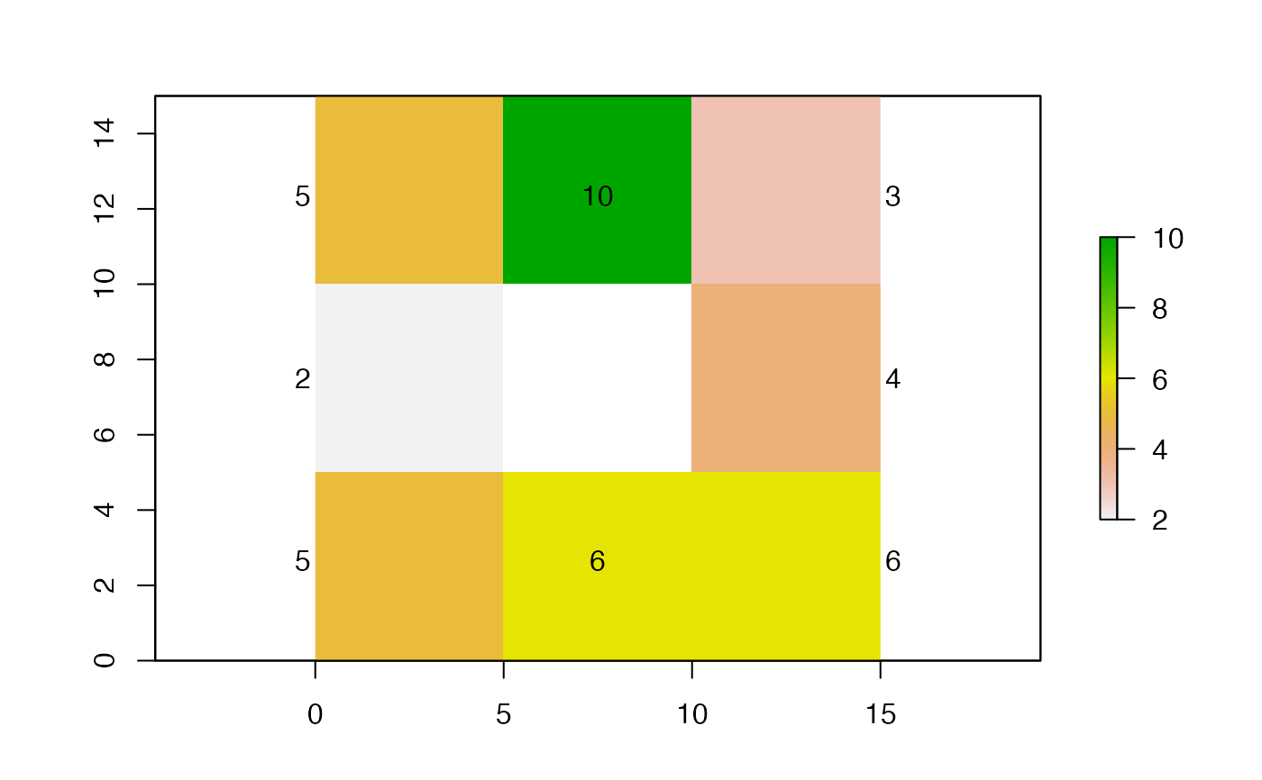
#### Example (4): Find the shortest distances around NAs
## Force the 5th cell to be NA
rtmp <- r
rtmp[5] <- NA
raster::plot(rtmp)
raster::text(rtmp)
#> [1] 13.95499
# shortest distance between cell 1 and 6 via cppRouting
lcp_over_surface(
origin = rxy[1, , drop = FALSE],
destination = rxy[6, , drop = FALSE],
surface = r,
method = "cppRouting",
verbose = FALSE
)$dist_lcp
#> Warning: transition function gives negative values
#> [1] 13.95499
## Compare to manually computed distances
# The shortest distance from cell 1 to cell 6 is to move diagonally
# ... from cell 1 to 5 and then 6.
# Define planar distances of moving like a rook (d_pr) or bishop (d_pb)
d_pr <- 5
d_pb <- sqrt(5^2 + 5^2)
# Define total distance travelled along shortest path, as computed by the
# ... algorithm to demonstrate we obtain the same value:
sqrt((5 - 1)^2 + d_pb^2) + sqrt((4 - 1)^2 + d_pr^2)
#> [1] 13.95499
#### Example (4): Find the shortest distances around NAs
## Force the 5th cell to be NA
rtmp <- r
rtmp[5] <- NA
raster::plot(rtmp)
raster::text(rtmp)
 ## Compute shortest distances via algorithm:
# Now compute shortest distances, which we can see have increased the distance
# ... since movement through an NA cell is not allowed. Therefore, if this NA
# ... reflects missing data, it may be appropriate to interpolate NAs using
# ... surrounding cells (e.g., see raster::approxNA()) so that movement
# ... is possible through these cells
out1 <- lcp_over_surface(
origin = rxy[1, , drop = FALSE],
destination = rxy[6, , drop = FALSE],
surface = rtmp,
method = "gdistance",
verbose = FALSE
)
#> Warning: transition function gives negative values
out2 <- lcp_over_surface(
origin = rxy[1, , drop = FALSE],
destination = rxy[6, , drop = FALSE],
surface = rtmp,
method = "cppRouting",
verbose = FALSE
)
#> Warning: transition function gives negative values
## Compute shortest distances via algorithm:
# Now compute shortest distances, which we can see have increased the distance
# ... since movement through an NA cell is not allowed. Therefore, if this NA
# ... reflects missing data, it may be appropriate to interpolate NAs using
# ... surrounding cells (e.g., see raster::approxNA()) so that movement
# ... is possible through these cells
out1 <- lcp_over_surface(
origin = rxy[1, , drop = FALSE],
destination = rxy[6, , drop = FALSE],
surface = rtmp,
method = "gdistance",
verbose = FALSE
)
#> Warning: transition function gives negative values
out2 <- lcp_over_surface(
origin = rxy[1, , drop = FALSE],
destination = rxy[6, , drop = FALSE],
surface = rtmp,
method = "cppRouting",
verbose = FALSE
)
#> Warning: transition function gives negative values
 out1$dist_lcp
#> [1] 16.34469
out2$dist_lcp
#> [1] 16.34469
## Compare to manual calculations of shortest route:
# Route option one: cell 1 to 2, 2 to 6
sqrt((5 - 10)^2 + d_pr^2) + sqrt((10 - 4)^2 + d_pb^2)
#> [1] 16.34469
# Or, using the numbers computed in the dist_total object:
out1$cost$dist_total[1, 2] + out1$cost$dist_total[2, 6]
#> [1] 16.34469
## Compare to effect of making a value in the landscape extremely large
# In the same way, we can force the shortest path away from particular areas
# ... by making the height of the landscape in those areas very large or Inf:
rtmp[5] <- 1e20
raster::plot(rtmp)
raster::text(rtmp)
out1$dist_lcp
#> [1] 16.34469
out2$dist_lcp
#> [1] 16.34469
## Compare to manual calculations of shortest route:
# Route option one: cell 1 to 2, 2 to 6
sqrt((5 - 10)^2 + d_pr^2) + sqrt((10 - 4)^2 + d_pb^2)
#> [1] 16.34469
# Or, using the numbers computed in the dist_total object:
out1$cost$dist_total[1, 2] + out1$cost$dist_total[2, 6]
#> [1] 16.34469
## Compare to effect of making a value in the landscape extremely large
# In the same way, we can force the shortest path away from particular areas
# ... by making the height of the landscape in those areas very large or Inf:
rtmp[5] <- 1e20
raster::plot(rtmp)
raster::text(rtmp)
 lcp_over_surface(
origin = rxy[1, , drop = FALSE],
destination = rxy[6, , drop = FALSE],
surface = rtmp,
method = "cppRouting",
verbose = FALSE
)$dist_lcp
#> Warning: transition function gives negative values
#> [1] 16.34469
lcp_over_surface(
origin = rxy[1, , drop = FALSE],
destination = rxy[6, , drop = FALSE],
surface = rtmp,
method = "gdistance",
verbose = FALSE
)$dist_lcp
#> Warning: transition function gives negative values
lcp_over_surface(
origin = rxy[1, , drop = FALSE],
destination = rxy[6, , drop = FALSE],
surface = rtmp,
method = "cppRouting",
verbose = FALSE
)$dist_lcp
#> Warning: transition function gives negative values
#> [1] 16.34469
lcp_over_surface(
origin = rxy[1, , drop = FALSE],
destination = rxy[6, , drop = FALSE],
surface = rtmp,
method = "gdistance",
verbose = FALSE
)$dist_lcp
#> Warning: transition function gives negative values
 #> [1] 16.34469
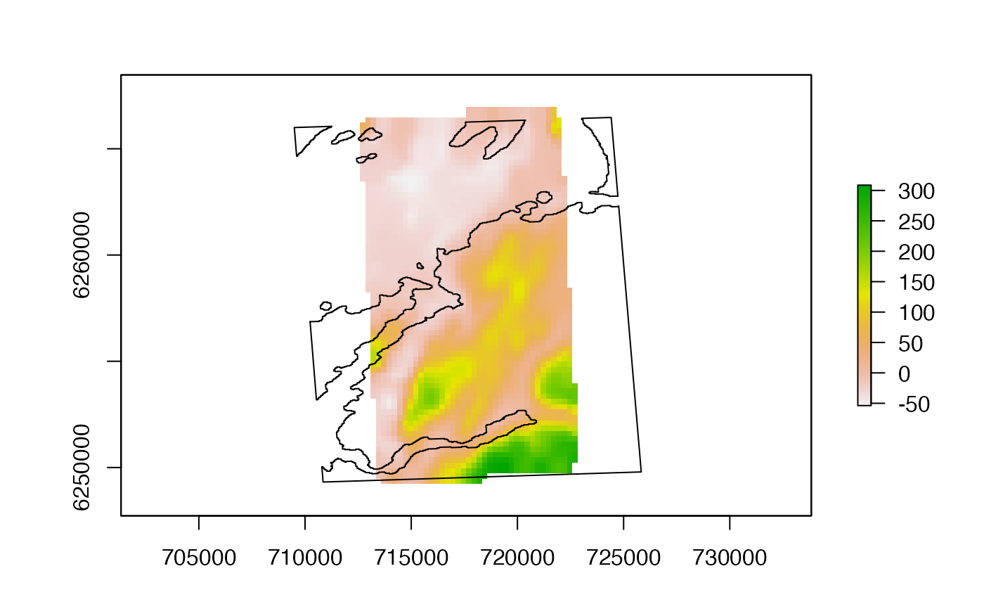
#### Example (4): Find the distances between points on a real landscape
## We will use some example bathymetry data:
dat_gebco_oban <- prettyGraphics::dat_gebco
raster::plot(dat_gebco_oban)
#> [1] 16.34469
#### Example (4): Find the distances between points on a real landscape
## We will use some example bathymetry data:
dat_gebco_oban <- prettyGraphics::dat_gebco
raster::plot(dat_gebco_oban)
 ## Process bathymetry data before function implementation
# (a) Define utm coordinates:
dat_gebco_utm <- raster::projectRaster(dat_gebco_oban, crs = proj_utm)
raster::res(dat_gebco_utm)
#> [1] 257 463
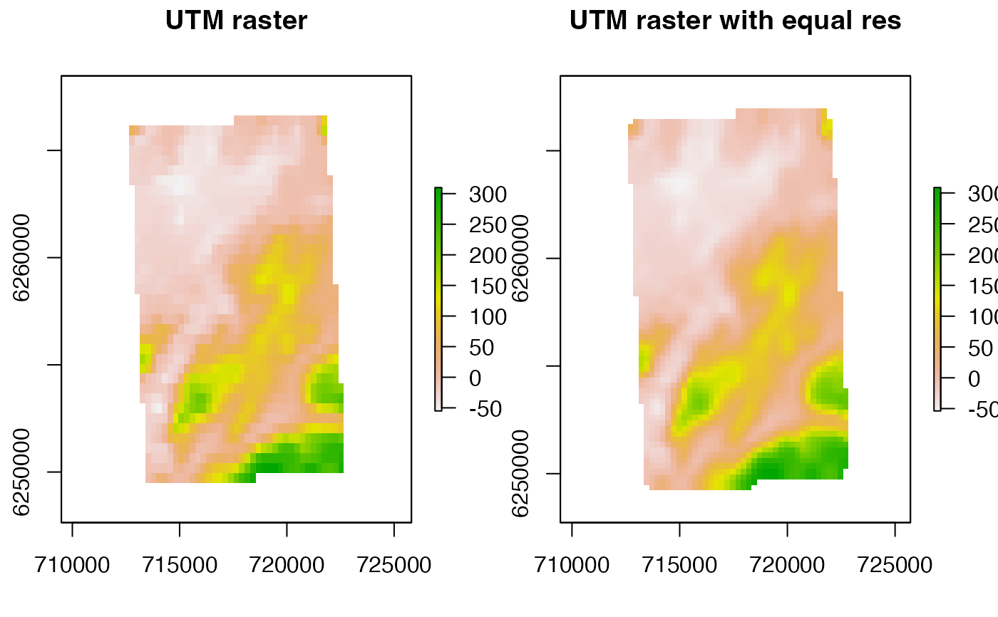
# (b) Resample so that the resolution in the x and y directions is identical
dat_gebco_utm_planar <- raster::raster(
crs = proj_utm,
ext = raster::extent(dat_gebco_utm),
resolution = 250
)
dat_gebco_utm_planar <- raster::resample(dat_gebco_utm, dat_gebco_utm_planar, method = "bilinear")
# Examine processed raster
pp <- par(mfrow = c(1, 2))
raster::plot(dat_gebco_utm, main = "UTM raster")
raster::plot(dat_gebco_utm_planar, main = "UTM raster with equal res")
## Process bathymetry data before function implementation
# (a) Define utm coordinates:
dat_gebco_utm <- raster::projectRaster(dat_gebco_oban, crs = proj_utm)
raster::res(dat_gebco_utm)
#> [1] 257 463
# (b) Resample so that the resolution in the x and y directions is identical
dat_gebco_utm_planar <- raster::raster(
crs = proj_utm,
ext = raster::extent(dat_gebco_utm),
resolution = 250
)
dat_gebco_utm_planar <- raster::resample(dat_gebco_utm, dat_gebco_utm_planar, method = "bilinear")
# Examine processed raster
pp <- par(mfrow = c(1, 2))
raster::plot(dat_gebco_utm, main = "UTM raster")
raster::plot(dat_gebco_utm_planar, main = "UTM raster with equal res")
 par(pp)
## Define example origin and destination
set.seed(1)
dat_gebco_utm_planar_xy <- raster::coordinates(dat_gebco_utm_planar)
index <- sample(1:nrow(dat_gebco_utm_planar_xy), 2)
origin <- dat_gebco_utm_planar_xy[index[1], , drop = FALSE]
destination <- dat_gebco_utm_planar_xy[index[2], , drop = FALSE]
## Implement function to compute shortest distances
out_gebco1 <- lcp_over_surface(
origin = origin,
destination = destination,
surface = dat_gebco_utm_planar,
method = "gdistance"
)
#> flapper::lcp_over_surface() called (@ 2023-08-29 15:43:59)...
#> ... Checking user inputs...
#> ... Defining cost matrix...
#> Warning: transition function gives negative values
par(pp)
## Define example origin and destination
set.seed(1)
dat_gebco_utm_planar_xy <- raster::coordinates(dat_gebco_utm_planar)
index <- sample(1:nrow(dat_gebco_utm_planar_xy), 2)
origin <- dat_gebco_utm_planar_xy[index[1], , drop = FALSE]
destination <- dat_gebco_utm_planar_xy[index[2], , drop = FALSE]
## Implement function to compute shortest distances
out_gebco1 <- lcp_over_surface(
origin = origin,
destination = destination,
surface = dat_gebco_utm_planar,
method = "gdistance"
)
#> flapper::lcp_over_surface() called (@ 2023-08-29 15:43:59)...
#> ... Checking user inputs...
#> ... Defining cost matrix...
#> Warning: transition function gives negative values
 #> ... Calculating Euclidean distance(s)...
#> ... Using method = 'gdistance'...
#> ... ... Defining 'ease' matrix...
#> ... ... Implementing Dijkstra's algorithm to compute least-cost distance(s)...
#> ... flapper::lcp_over_surface() call completed (@ 2023-08-29 15:43:59) after ~0 minutes.
out_gebco2 <- lcp_over_surface(
origin = origin,
destination = destination,
surface = dat_gebco_utm_planar,
method = "cppRouting"
)
#> flapper::lcp_over_surface() called (@ 2023-08-29 15:43:59)...
#> ... Checking user inputs...
#> ... Defining cost matrix...
#> Warning: transition function gives negative values
#> ... Calculating Euclidean distance(s)...
#> ... Using method = 'cppRouting'...
#> ... ... Defining nodes, edges and costs to make graph...
#> ... ... Constructing graph object...
#> ... ... Implementing bi algorithm to compute least-cost distance(s)...
#> ... flapper::lcp_over_surface() call completed (@ 2023-08-29 15:43:59) after ~0.01 minutes.
# Compare Euclidean and shortest distances
out_gebco1$dist_euclid
#> [1] 8902.247
out_gebco1$dist_lcp
#> [1] 9278.626
out_gebco2$dist_euclid
#> [1] 8902.247
out_gebco2$dist_lcp
#> [1] 9278.626
#### Example (5A): Reduce the complexity of the landscape by cropping
ext <- raster::extent(dat_gebco_utm_planar)
ext[3] <- 6255000
ext[4] <- 6265000
out_gebco1 <- lcp_over_surface(
origin = origin,
destination = destination,
surface = dat_gebco_utm_planar,
method = "gdistance",
crop = ext
)
#> flapper::lcp_over_surface() called (@ 2023-08-29 15:43:59)...
#> ... Checking user inputs...
#> ... Cropping raster to inputted extent...
#> ... Defining cost matrix...
#> Warning: transition function gives negative values
#> ... Calculating Euclidean distance(s)...
#> ... Using method = 'gdistance'...
#> ... ... Defining 'ease' matrix...
#> ... ... Implementing Dijkstra's algorithm to compute least-cost distance(s)...
#> ... flapper::lcp_over_surface() call completed (@ 2023-08-29 15:43:59) after ~0 minutes.
out_gebco2 <- lcp_over_surface(
origin = origin,
destination = destination,
surface = dat_gebco_utm_planar,
method = "cppRouting"
)
#> flapper::lcp_over_surface() called (@ 2023-08-29 15:43:59)...
#> ... Checking user inputs...
#> ... Defining cost matrix...
#> Warning: transition function gives negative values
#> ... Calculating Euclidean distance(s)...
#> ... Using method = 'cppRouting'...
#> ... ... Defining nodes, edges and costs to make graph...
#> ... ... Constructing graph object...
#> ... ... Implementing bi algorithm to compute least-cost distance(s)...
#> ... flapper::lcp_over_surface() call completed (@ 2023-08-29 15:43:59) after ~0.01 minutes.
# Compare Euclidean and shortest distances
out_gebco1$dist_euclid
#> [1] 8902.247
out_gebco1$dist_lcp
#> [1] 9278.626
out_gebco2$dist_euclid
#> [1] 8902.247
out_gebco2$dist_lcp
#> [1] 9278.626
#### Example (5A): Reduce the complexity of the landscape by cropping
ext <- raster::extent(dat_gebco_utm_planar)
ext[3] <- 6255000
ext[4] <- 6265000
out_gebco1 <- lcp_over_surface(
origin = origin,
destination = destination,
surface = dat_gebco_utm_planar,
method = "gdistance",
crop = ext
)
#> flapper::lcp_over_surface() called (@ 2023-08-29 15:43:59)...
#> ... Checking user inputs...
#> ... Cropping raster to inputted extent...
#> ... Defining cost matrix...
#> Warning: transition function gives negative values
 #> ... Calculating Euclidean distance(s)...
#> ... Using method = 'gdistance'...
#> ... ... Defining 'ease' matrix...
#> ... ... Implementing Dijkstra's algorithm to compute least-cost distance(s)...
#> ... flapper::lcp_over_surface() call completed (@ 2023-08-29 15:44:00) after ~0 minutes.
out_gebco1$dist_lcp
#> [1] 9278.626
#### Example (5B): Reduce the complexity of the landscape around a buffer
out_gebco1 <- lcp_over_surface(
origin = origin,
destination = destination,
surface = dat_gebco_utm_planar,
method = "gdistance",
buffer = list(width = 1000)
)
#> flapper::lcp_over_surface() called (@ 2023-08-29 15:44:00)...
#> ... Checking user inputs...
#> ... Cropping raster to buffer zone around a Euclidean transect between the origin and destination...
#> Warning: GEOS support is provided by the sf and terra packages among others
#> ... Defining cost matrix...
#> Warning: transition function gives negative values
#> ... Calculating Euclidean distance(s)...
#> ... Using method = 'gdistance'...
#> ... ... Defining 'ease' matrix...
#> ... ... Implementing Dijkstra's algorithm to compute least-cost distance(s)...
#> ... flapper::lcp_over_surface() call completed (@ 2023-08-29 15:44:00) after ~0 minutes.
out_gebco1$dist_lcp
#> [1] 9278.626
#### Example (5B): Reduce the complexity of the landscape around a buffer
out_gebco1 <- lcp_over_surface(
origin = origin,
destination = destination,
surface = dat_gebco_utm_planar,
method = "gdistance",
buffer = list(width = 1000)
)
#> flapper::lcp_over_surface() called (@ 2023-08-29 15:44:00)...
#> ... Checking user inputs...
#> ... Cropping raster to buffer zone around a Euclidean transect between the origin and destination...
#> Warning: GEOS support is provided by the sf and terra packages among others
#> ... Defining cost matrix...
#> Warning: transition function gives negative values
 #> ... Calculating Euclidean distance(s)...
#> ... Using method = 'gdistance'...
#> ... ... Defining 'ease' matrix...
#> ... ... Implementing Dijkstra's algorithm to compute least-cost distance(s)...
#> ... flapper::lcp_over_surface() call completed (@ 2023-08-29 15:44:00) after ~0 minutes.
out_gebco1$dist_lcp
#> [1] 9278.626
#### Example (5C): Reduce the complexity of the landscape via aggregation
out_gebco1 <- lcp_over_surface(
origin = origin,
destination = destination,
surface = dat_gebco_utm_planar,
method = "gdistance",
buffer = list(width = 1000),
aggregate = list(fact = 5, fun = mean, na.rm = TRUE)
)
#> flapper::lcp_over_surface() called (@ 2023-08-29 15:44:00)...
#> ... Checking user inputs...
#> ... Cropping raster to buffer zone around a Euclidean transect between the origin and destination...
#> Warning: GEOS support is provided by the sf and terra packages among others
#> ... Aggregating raster...
#> ... Defining cost matrix...
#> Warning: transition function gives negative values
#> ... Calculating Euclidean distance(s)...
#> ... Using method = 'gdistance'...
#> ... ... Defining 'ease' matrix...
#> ... ... Implementing Dijkstra's algorithm to compute least-cost distance(s)...
#> ... flapper::lcp_over_surface() call completed (@ 2023-08-29 15:44:00) after ~0 minutes.
out_gebco1$dist_lcp
#> [1] 9278.626
#### Example (5C): Reduce the complexity of the landscape via aggregation
out_gebco1 <- lcp_over_surface(
origin = origin,
destination = destination,
surface = dat_gebco_utm_planar,
method = "gdistance",
buffer = list(width = 1000),
aggregate = list(fact = 5, fun = mean, na.rm = TRUE)
)
#> flapper::lcp_over_surface() called (@ 2023-08-29 15:44:00)...
#> ... Checking user inputs...
#> ... Cropping raster to buffer zone around a Euclidean transect between the origin and destination...
#> Warning: GEOS support is provided by the sf and terra packages among others
#> ... Aggregating raster...
#> ... Defining cost matrix...
#> Warning: transition function gives negative values
 #> ... Calculating Euclidean distance(s)...
#> ... Using method = 'gdistance'...
#> ... ... Defining 'ease' matrix...
#> ... ... Implementing Dijkstra's algorithm to compute least-cost distance(s)...
#> ... flapper::lcp_over_surface() call completed (@ 2023-08-29 15:44:00) after ~0 minutes.
out_gebco1$dist_lcp
#> [1] 10088.96
#### Example (6C): Implement a mask
# Define coastline
dat_coast_around_oban <- prettyGraphics::dat_coast_around_oban
coastline <- sp::spTransform(dat_coast_around_oban, proj_utm)
# Visualise bathymetry and coastline
raster::plot(dat_gebco_utm_planar)
raster::lines(coastline)
#> ... Calculating Euclidean distance(s)...
#> ... Using method = 'gdistance'...
#> ... ... Defining 'ease' matrix...
#> ... ... Implementing Dijkstra's algorithm to compute least-cost distance(s)...
#> ... flapper::lcp_over_surface() call completed (@ 2023-08-29 15:44:00) after ~0 minutes.
out_gebco1$dist_lcp
#> [1] 10088.96
#### Example (6C): Implement a mask
# Define coastline
dat_coast_around_oban <- prettyGraphics::dat_coast_around_oban
coastline <- sp::spTransform(dat_coast_around_oban, proj_utm)
# Visualise bathymetry and coastline
raster::plot(dat_gebco_utm_planar)
raster::lines(coastline)
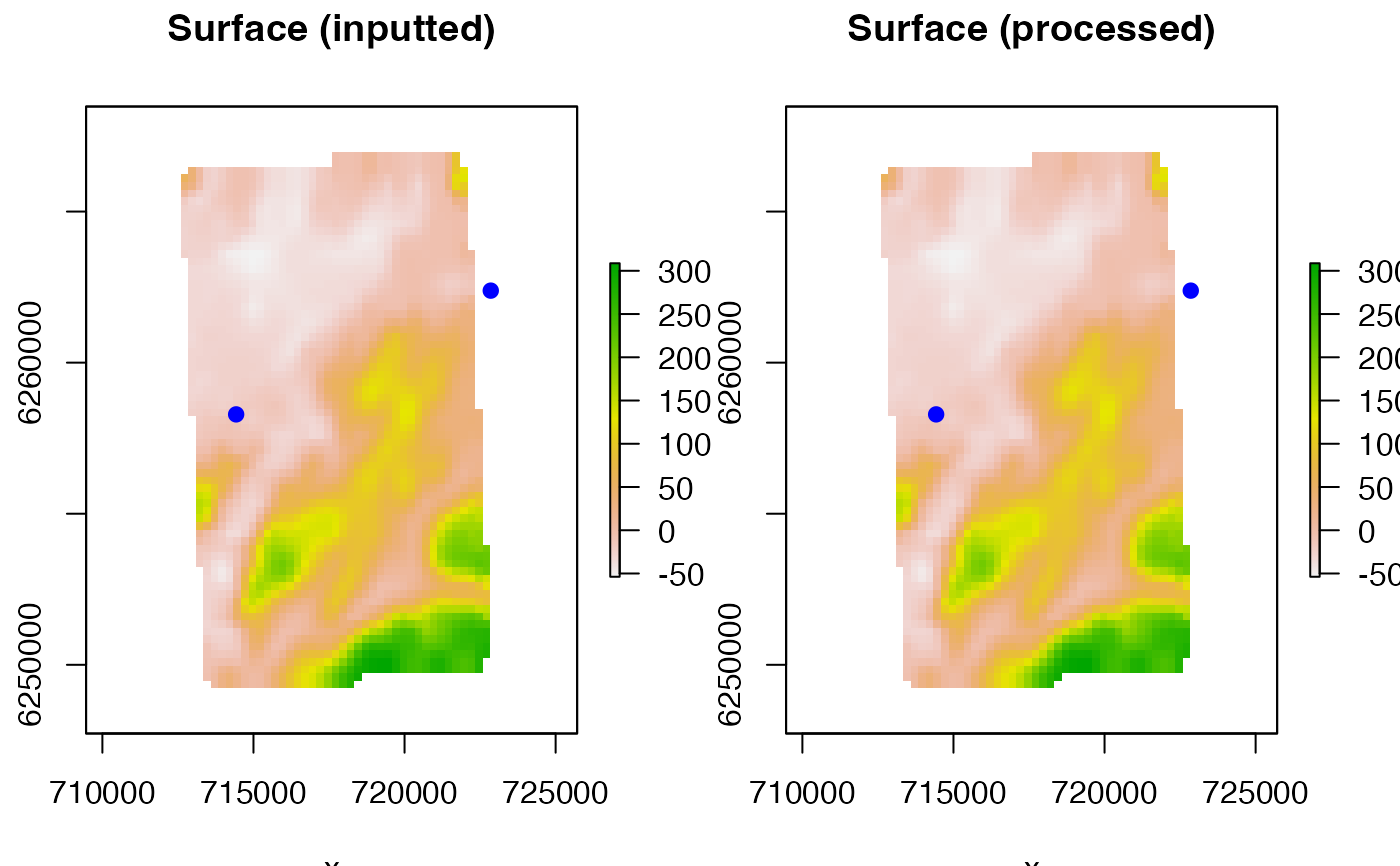
 # Define example origin and destination within the sea
origin <- matrix(c(714000, 6260000), ncol = 2)
destination <- matrix(c(721000, 6265000), ncol = 2)
# Implement algorithm
out_gebco1 <- lcp_over_surface(
origin = origin,
destination = destination,
surface = dat_gebco_utm_planar,
method = "gdistance",
crop = raster::extent(coastline),
mask = coastline,
mask_inside = TRUE
)
#> flapper::lcp_over_surface() called (@ 2023-08-29 15:44:00)...
#> ... Checking user inputs...
#> ... Cropping raster to inputted extent...
#> ... Masking raster...
#> Warning: GEOS support is provided by the sf and terra packages among others
#> ... Defining cost matrix...
#> Warning: transition function gives negative values
#> ... Calculating Euclidean distance(s)...
#> ... Using method = 'gdistance'...
#> ... ... Defining 'ease' matrix...
#> ... ... Implementing Dijkstra's algorithm to compute least-cost distance(s)...
#> ... flapper::lcp_over_surface() call completed (@ 2023-08-29 15:44:00) after ~0 minutes.
out_gebco2 <- lcp_over_surface(
origin = origin,
destination = destination,
surface = dat_gebco_utm_planar,
method = "cppRouting",
crop = raster::extent(coastline),
mask = coastline,
mask_inside = TRUE
)
#> flapper::lcp_over_surface() called (@ 2023-08-29 15:44:00)...
#> ... Checking user inputs...
#> ... Cropping raster to inputted extent...
#> ... Masking raster...
#> Warning: GEOS support is provided by the sf and terra packages among others
#> ... Defining cost matrix...
#> Warning: transition function gives negative values
# Define example origin and destination within the sea
origin <- matrix(c(714000, 6260000), ncol = 2)
destination <- matrix(c(721000, 6265000), ncol = 2)
# Implement algorithm
out_gebco1 <- lcp_over_surface(
origin = origin,
destination = destination,
surface = dat_gebco_utm_planar,
method = "gdistance",
crop = raster::extent(coastline),
mask = coastline,
mask_inside = TRUE
)
#> flapper::lcp_over_surface() called (@ 2023-08-29 15:44:00)...
#> ... Checking user inputs...
#> ... Cropping raster to inputted extent...
#> ... Masking raster...
#> Warning: GEOS support is provided by the sf and terra packages among others
#> ... Defining cost matrix...
#> Warning: transition function gives negative values
#> ... Calculating Euclidean distance(s)...
#> ... Using method = 'gdistance'...
#> ... ... Defining 'ease' matrix...
#> ... ... Implementing Dijkstra's algorithm to compute least-cost distance(s)...
#> ... flapper::lcp_over_surface() call completed (@ 2023-08-29 15:44:00) after ~0 minutes.
out_gebco2 <- lcp_over_surface(
origin = origin,
destination = destination,
surface = dat_gebco_utm_planar,
method = "cppRouting",
crop = raster::extent(coastline),
mask = coastline,
mask_inside = TRUE
)
#> flapper::lcp_over_surface() called (@ 2023-08-29 15:44:00)...
#> ... Checking user inputs...
#> ... Cropping raster to inputted extent...
#> ... Masking raster...
#> Warning: GEOS support is provided by the sf and terra packages among others
#> ... Defining cost matrix...
#> Warning: transition function gives negative values
 #> ... Calculating Euclidean distance(s)...
#> ... Using method = 'cppRouting'...
#> ... ... Defining nodes, edges and costs to make graph...
#> ... ... Constructing graph object...
#> ... ... Implementing bi algorithm to compute least-cost distance(s)...
#> ... flapper::lcp_over_surface() call completed (@ 2023-08-29 15:44:01) after ~0.01 minutes.
# Compare Euclidean and least-cost distances
out_gebco1$dist_euclid
#> [1] 8602.325
out_gebco1$dist_lcp
#> [1] 9071.48
out_gebco2$dist_euclid
#> [1] 8602.325
out_gebco2$dist_lcp
#> [1] 9071.48
#### Example (7) Implement shortest distance algorithms in parallel:
# With the default method ("cppRouting"), use use_all_cores = TRUE
out_gebco1 <- lcp_over_surface(
origin = origin,
destination = destination,
surface = dat_gebco_utm_planar,
method = "cppRouting",
crop = raster::extent(coastline),
mask = coastline,
mask_inside = TRUE,
use_all_cores = TRUE
)
#> flapper::lcp_over_surface() called (@ 2023-08-29 15:44:01)...
#> ... Checking user inputs...
#> ... Cropping raster to inputted extent...
#> ... Masking raster...
#> Warning: GEOS support is provided by the sf and terra packages among others
#> ... Defining cost matrix...
#> Warning: transition function gives negative values
#> ... Calculating Euclidean distance(s)...
#> ... Using method = 'cppRouting'...
#> ... ... Defining nodes, edges and costs to make graph...
#> ... ... Constructing graph object...
#> ... ... Implementing bi algorithm to compute least-cost distance(s)...
#> allcores argument is deprecated since v3.0.
#> Please use RcppParallel::setThreadOptions() to set the number of threads
#> ... flapper::lcp_over_surface() call completed (@ 2023-08-29 15:44:01) after ~0 minutes.
# With method = "gdistance" use cl argument
out_gebco2 <- lcp_over_surface(
origin = origin,
destination = destination,
surface = dat_gebco_utm_planar,
method = "cppRouting",
crop = raster::extent(coastline),
mask = coastline,
mask_inside = TRUE,
cl = parallel::makeCluster(2L)
)
#> flapper::lcp_over_surface() called (@ 2023-08-29 15:44:01)...
#> ... Checking user inputs...
#> 'cl' or 'varlist' arguments ignored for method = 'cppRouting': use use_all_cores = TRUE instead.
#> ... Cropping raster to inputted extent...
#> ... Masking raster...
#> Warning: GEOS support is provided by the sf and terra packages among others
#> ... Defining cost matrix...
#> Warning: transition function gives negative values
#> ... Calculating Euclidean distance(s)...
#> ... Using method = 'cppRouting'...
#> ... ... Defining nodes, edges and costs to make graph...
#> ... ... Constructing graph object...
#> ... ... Implementing bi algorithm to compute least-cost distance(s)...
#> ... flapper::lcp_over_surface() call completed (@ 2023-08-29 15:44:02) after ~0.01 minutes.
out_gebco1$dist_lcp
#> [1] 9071.48
out_gebco2$dist_lcp
#> [1] 9071.48
############################################################################
#### Shortest paths between a single origin and a single destination
#### Example (8) Shortest paths (goal = 2) only using default method
# Implement function
out1 <- lcp_over_surface(
origin = rxy[1, , drop = FALSE],
destination = rxy[6, , drop = FALSE],
surface = r,
goal = 2
)
#> flapper::lcp_over_surface() called (@ 2023-08-29 15:44:02)...
#> ... Checking user inputs...
#> ... Defining cost matrix...
#> Warning: transition function gives negative values
#> ... Using method = 'cppRouting'...
#> ... ... Defining nodes, edges and costs to make graph...
#> ... ... Constructing graph object...
#> ... ... Implementing bi algorithm to compute least-cost paths(s)...
#> ... flapper::lcp_over_surface() call completed (@ 2023-08-29 15:44:02) after ~0 minutes.
# The path is stored in path_lcp, This includes:
# ... (a) a dataframe with the cells comprising each path:
# ... (b) a SpatialLines object of the path
# ... (c) a matrix of the coordinates of the path
out1$path_lcp
#> $cells
#> path_id path origin destination cell
#> 1 1 1-6 1 6 6
#> 2 1 1-6 1 6 5
#> 3 1 1-6 1 6 1
#>
#> $SpatialLines
#> $SpatialLines$`1`
#> class : SpatialLines
#> features : 1
#> extent : 2.5, 12.5, 7.5, 12.5 (xmin, xmax, ymin, ymax)
#> crs : +proj=utm +zone=29 +datum=WGS84 +units=m +no_defs
#>
#>
#> $coordinates
#> $coordinates$`1`
#> x y
#> [1,] 12.5 7.5
#> [2,] 7.5 7.5
#> [3,] 2.5 12.5
#>
#>
# For method = "cppRouting", paths between pairs of coordinates are computed
# ... by cppRouting::get_path_pair(), the arguments of which are retained in
# ... this list:
out1$cppRouting_param$get_path_pair_param
#> $Graph
#> $Graph$data
#> from to dist
#> 1 0 3 7.071068
#> 2 1 3 5.830952
#> 3 2 3 8.124038
#> 4 3 0 7.071068
#> 5 4 0 8.602325
#> 6 1 0 10.677078
#> 7 2 0 10.295630
#> 8 5 0 9.273618
#> 9 0 4 8.602325
#> 10 2 4 7.348469
#> 11 5 4 5.099020
#> 12 3 1 5.830952
#> 13 0 1 10.677078
#> 14 2 1 5.099020
#> 15 6 1 5.830952
#> 16 7 1 8.124038
#> 17 3 2 8.124038
#> 18 0 2 10.295630
#> 19 4 2 7.348469
#> 20 1 2 5.099020
#> 21 5 2 5.830952
#> 22 6 2 8.124038
#> 23 7 2 7.071068
#> 24 8 2 8.660254
#> 25 0 5 9.273618
#> 26 4 5 5.099020
#> 27 2 5 5.830952
#> 28 7 5 7.348469
#> 29 8 5 5.385165
#> 30 1 6 5.830952
#> 31 2 6 8.124038
#> 32 7 6 5.099020
#> 33 1 7 8.124038
#> 34 2 7 7.071068
#> 35 5 7 7.348469
#> 36 6 7 5.099020
#> 37 8 7 5.000000
#> 38 2 8 8.660254
#> 39 5 8 5.385165
#> 40 7 8 5.000000
#> 41 3 0 7.071068
#> 42 3 1 5.830952
#> 43 3 2 8.124038
#> 44 0 3 7.071068
#> 45 0 4 8.602325
#> 46 0 1 10.677078
#> 47 0 2 10.295630
#> 48 0 5 9.273618
#> 49 4 0 8.602325
#> 50 4 2 7.348469
#> 51 4 5 5.099020
#> 52 1 3 5.830952
#> 53 1 0 10.677078
#> 54 1 2 5.099020
#> 55 1 6 5.830952
#> 56 1 7 8.124038
#> 57 2 3 8.124038
#> 58 2 0 10.295630
#> 59 2 4 7.348469
#> 60 2 1 5.099020
#> 61 2 5 5.830952
#> 62 2 6 8.124038
#> 63 2 7 7.071068
#> 64 2 8 8.660254
#> 65 5 0 9.273618
#> 66 5 4 5.099020
#> 67 5 2 5.830952
#> 68 5 7 7.348469
#> 69 5 8 5.385165
#> 70 6 1 5.830952
#> 71 6 2 8.124038
#> 72 6 7 5.099020
#> 73 7 1 8.124038
#> 74 7 2 7.071068
#> 75 7 5 7.348469
#> 76 7 6 5.099020
#> 77 7 8 5.000000
#> 78 8 2 8.660254
#> 79 8 5 5.385165
#> 80 8 7 5.000000
#>
#> $Graph$coords
#> node X Y
#> 2 2 7.5 12.5
#> 4 4 2.5 7.5
#> 5 5 7.5 7.5
#> 1 1 2.5 12.5
#> 3 3 12.5 12.5
#> 6 6 12.5 7.5
#> 7 7 2.5 2.5
#> 8 8 7.5 2.5
#> 9 9 12.5 2.5
#>
#> $Graph$nbnode
#> [1] 9
#>
#> $Graph$dict
#> ref id
#> 1 2 0
#> 2 4 1
#> 3 5 2
#> 4 1 3
#> 5 3 4
#> 6 6 5
#> 7 7 6
#> 8 8 7
#> 9 9 8
#>
#> $Graph$attrib
#> $Graph$attrib$aux
#> NULL
#>
#> $Graph$attrib$cap
#> NULL
#>
#> $Graph$attrib$alpha
#> NULL
#>
#> $Graph$attrib$beta
#> NULL
#>
#>
#>
#> $from
#> [1] 1
#>
#> $to
#> [1] 6
#>
#> $algorithm
#> [1] "bi"
#>
#> $constant
#> [1] 1
#>
#> $keep
#> NULL
#>
#> $long
#> [1] TRUE
#>
# Note the path is also added to the plot produced, if plot = TRUE.
#### Example (9) Shortest distances and paths (goal = 3) using default method
out1 <- lcp_over_surface(
origin = rxy[1, , drop = FALSE],
destination = rxy[6, , drop = FALSE],
surface = r,
goal = 3
)
#> flapper::lcp_over_surface() called (@ 2023-08-29 15:44:02)...
#> ... Checking user inputs...
#> ... Defining cost matrix...
#> Warning: transition function gives negative values
#> ... Calculating Euclidean distance(s)...
#> ... Using method = 'cppRouting'...
#> ... ... Defining nodes, edges and costs to make graph...
#> ... ... Constructing graph object...
#> ... ... Implementing bi algorithm to compute least-cost distance(s)...
#> ... flapper::lcp_over_surface() call completed (@ 2023-08-29 15:44:01) after ~0.01 minutes.
# Compare Euclidean and least-cost distances
out_gebco1$dist_euclid
#> [1] 8602.325
out_gebco1$dist_lcp
#> [1] 9071.48
out_gebco2$dist_euclid
#> [1] 8602.325
out_gebco2$dist_lcp
#> [1] 9071.48
#### Example (7) Implement shortest distance algorithms in parallel:
# With the default method ("cppRouting"), use use_all_cores = TRUE
out_gebco1 <- lcp_over_surface(
origin = origin,
destination = destination,
surface = dat_gebco_utm_planar,
method = "cppRouting",
crop = raster::extent(coastline),
mask = coastline,
mask_inside = TRUE,
use_all_cores = TRUE
)
#> flapper::lcp_over_surface() called (@ 2023-08-29 15:44:01)...
#> ... Checking user inputs...
#> ... Cropping raster to inputted extent...
#> ... Masking raster...
#> Warning: GEOS support is provided by the sf and terra packages among others
#> ... Defining cost matrix...
#> Warning: transition function gives negative values
#> ... Calculating Euclidean distance(s)...
#> ... Using method = 'cppRouting'...
#> ... ... Defining nodes, edges and costs to make graph...
#> ... ... Constructing graph object...
#> ... ... Implementing bi algorithm to compute least-cost distance(s)...
#> allcores argument is deprecated since v3.0.
#> Please use RcppParallel::setThreadOptions() to set the number of threads
#> ... flapper::lcp_over_surface() call completed (@ 2023-08-29 15:44:01) after ~0 minutes.
# With method = "gdistance" use cl argument
out_gebco2 <- lcp_over_surface(
origin = origin,
destination = destination,
surface = dat_gebco_utm_planar,
method = "cppRouting",
crop = raster::extent(coastline),
mask = coastline,
mask_inside = TRUE,
cl = parallel::makeCluster(2L)
)
#> flapper::lcp_over_surface() called (@ 2023-08-29 15:44:01)...
#> ... Checking user inputs...
#> 'cl' or 'varlist' arguments ignored for method = 'cppRouting': use use_all_cores = TRUE instead.
#> ... Cropping raster to inputted extent...
#> ... Masking raster...
#> Warning: GEOS support is provided by the sf and terra packages among others
#> ... Defining cost matrix...
#> Warning: transition function gives negative values
#> ... Calculating Euclidean distance(s)...
#> ... Using method = 'cppRouting'...
#> ... ... Defining nodes, edges and costs to make graph...
#> ... ... Constructing graph object...
#> ... ... Implementing bi algorithm to compute least-cost distance(s)...
#> ... flapper::lcp_over_surface() call completed (@ 2023-08-29 15:44:02) after ~0.01 minutes.
out_gebco1$dist_lcp
#> [1] 9071.48
out_gebco2$dist_lcp
#> [1] 9071.48
############################################################################
#### Shortest paths between a single origin and a single destination
#### Example (8) Shortest paths (goal = 2) only using default method
# Implement function
out1 <- lcp_over_surface(
origin = rxy[1, , drop = FALSE],
destination = rxy[6, , drop = FALSE],
surface = r,
goal = 2
)
#> flapper::lcp_over_surface() called (@ 2023-08-29 15:44:02)...
#> ... Checking user inputs...
#> ... Defining cost matrix...
#> Warning: transition function gives negative values
#> ... Using method = 'cppRouting'...
#> ... ... Defining nodes, edges and costs to make graph...
#> ... ... Constructing graph object...
#> ... ... Implementing bi algorithm to compute least-cost paths(s)...
#> ... flapper::lcp_over_surface() call completed (@ 2023-08-29 15:44:02) after ~0 minutes.
# The path is stored in path_lcp, This includes:
# ... (a) a dataframe with the cells comprising each path:
# ... (b) a SpatialLines object of the path
# ... (c) a matrix of the coordinates of the path
out1$path_lcp
#> $cells
#> path_id path origin destination cell
#> 1 1 1-6 1 6 6
#> 2 1 1-6 1 6 5
#> 3 1 1-6 1 6 1
#>
#> $SpatialLines
#> $SpatialLines$`1`
#> class : SpatialLines
#> features : 1
#> extent : 2.5, 12.5, 7.5, 12.5 (xmin, xmax, ymin, ymax)
#> crs : +proj=utm +zone=29 +datum=WGS84 +units=m +no_defs
#>
#>
#> $coordinates
#> $coordinates$`1`
#> x y
#> [1,] 12.5 7.5
#> [2,] 7.5 7.5
#> [3,] 2.5 12.5
#>
#>
# For method = "cppRouting", paths between pairs of coordinates are computed
# ... by cppRouting::get_path_pair(), the arguments of which are retained in
# ... this list:
out1$cppRouting_param$get_path_pair_param
#> $Graph
#> $Graph$data
#> from to dist
#> 1 0 3 7.071068
#> 2 1 3 5.830952
#> 3 2 3 8.124038
#> 4 3 0 7.071068
#> 5 4 0 8.602325
#> 6 1 0 10.677078
#> 7 2 0 10.295630
#> 8 5 0 9.273618
#> 9 0 4 8.602325
#> 10 2 4 7.348469
#> 11 5 4 5.099020
#> 12 3 1 5.830952
#> 13 0 1 10.677078
#> 14 2 1 5.099020
#> 15 6 1 5.830952
#> 16 7 1 8.124038
#> 17 3 2 8.124038
#> 18 0 2 10.295630
#> 19 4 2 7.348469
#> 20 1 2 5.099020
#> 21 5 2 5.830952
#> 22 6 2 8.124038
#> 23 7 2 7.071068
#> 24 8 2 8.660254
#> 25 0 5 9.273618
#> 26 4 5 5.099020
#> 27 2 5 5.830952
#> 28 7 5 7.348469
#> 29 8 5 5.385165
#> 30 1 6 5.830952
#> 31 2 6 8.124038
#> 32 7 6 5.099020
#> 33 1 7 8.124038
#> 34 2 7 7.071068
#> 35 5 7 7.348469
#> 36 6 7 5.099020
#> 37 8 7 5.000000
#> 38 2 8 8.660254
#> 39 5 8 5.385165
#> 40 7 8 5.000000
#> 41 3 0 7.071068
#> 42 3 1 5.830952
#> 43 3 2 8.124038
#> 44 0 3 7.071068
#> 45 0 4 8.602325
#> 46 0 1 10.677078
#> 47 0 2 10.295630
#> 48 0 5 9.273618
#> 49 4 0 8.602325
#> 50 4 2 7.348469
#> 51 4 5 5.099020
#> 52 1 3 5.830952
#> 53 1 0 10.677078
#> 54 1 2 5.099020
#> 55 1 6 5.830952
#> 56 1 7 8.124038
#> 57 2 3 8.124038
#> 58 2 0 10.295630
#> 59 2 4 7.348469
#> 60 2 1 5.099020
#> 61 2 5 5.830952
#> 62 2 6 8.124038
#> 63 2 7 7.071068
#> 64 2 8 8.660254
#> 65 5 0 9.273618
#> 66 5 4 5.099020
#> 67 5 2 5.830952
#> 68 5 7 7.348469
#> 69 5 8 5.385165
#> 70 6 1 5.830952
#> 71 6 2 8.124038
#> 72 6 7 5.099020
#> 73 7 1 8.124038
#> 74 7 2 7.071068
#> 75 7 5 7.348469
#> 76 7 6 5.099020
#> 77 7 8 5.000000
#> 78 8 2 8.660254
#> 79 8 5 5.385165
#> 80 8 7 5.000000
#>
#> $Graph$coords
#> node X Y
#> 2 2 7.5 12.5
#> 4 4 2.5 7.5
#> 5 5 7.5 7.5
#> 1 1 2.5 12.5
#> 3 3 12.5 12.5
#> 6 6 12.5 7.5
#> 7 7 2.5 2.5
#> 8 8 7.5 2.5
#> 9 9 12.5 2.5
#>
#> $Graph$nbnode
#> [1] 9
#>
#> $Graph$dict
#> ref id
#> 1 2 0
#> 2 4 1
#> 3 5 2
#> 4 1 3
#> 5 3 4
#> 6 6 5
#> 7 7 6
#> 8 8 7
#> 9 9 8
#>
#> $Graph$attrib
#> $Graph$attrib$aux
#> NULL
#>
#> $Graph$attrib$cap
#> NULL
#>
#> $Graph$attrib$alpha
#> NULL
#>
#> $Graph$attrib$beta
#> NULL
#>
#>
#>
#> $from
#> [1] 1
#>
#> $to
#> [1] 6
#>
#> $algorithm
#> [1] "bi"
#>
#> $constant
#> [1] 1
#>
#> $keep
#> NULL
#>
#> $long
#> [1] TRUE
#>
# Note the path is also added to the plot produced, if plot = TRUE.
#### Example (9) Shortest distances and paths (goal = 3) using default method
out1 <- lcp_over_surface(
origin = rxy[1, , drop = FALSE],
destination = rxy[6, , drop = FALSE],
surface = r,
goal = 3
)
#> flapper::lcp_over_surface() called (@ 2023-08-29 15:44:02)...
#> ... Checking user inputs...
#> ... Defining cost matrix...
#> Warning: transition function gives negative values
 #> ... Calculating Euclidean distance(s)...
#> ... Using method = 'cppRouting'...
#> ... ... Defining nodes, edges and costs to make graph...
#> ... ... Constructing graph object...
#> ... ... Implementing bi algorithm to compute least-cost distance(s)...
#> ... ... Implementing bi algorithm to compute least-cost paths(s)...
#> ... flapper::lcp_over_surface() call completed (@ 2023-08-29 15:44:02) after ~0 minutes.
out1$dist_lcp
#> [1] 13.95499
out1$path_lcp
#> $cells
#> path_id path origin destination cell
#> 1 1 1-6 1 6 6
#> 2 1 1-6 1 6 5
#> 3 1 1-6 1 6 1
#>
#> $SpatialLines
#> $SpatialLines$`1`
#> class : SpatialLines
#> features : 1
#> extent : 2.5, 12.5, 7.5, 12.5 (xmin, xmax, ymin, ymax)
#> crs : +proj=utm +zone=29 +datum=WGS84 +units=m +no_defs
#>
#>
#> $coordinates
#> $coordinates$`1`
#> x y
#> [1,] 12.5 7.5
#> [2,] 7.5 7.5
#> [3,] 2.5 12.5
#>
#>
#### Example (10) Shortest distances and paths (goal = 3) via gdistance
out1 <- lcp_over_surface(
origin = rxy[1, , drop = FALSE],
destination = rxy[6, , drop = FALSE],
surface = r,
goal = 3,
method = "gdistance"
)
#> flapper::lcp_over_surface() called (@ 2023-08-29 15:44:02)...
#> ... Checking user inputs...
#> ... Defining cost matrix...
#> Warning: transition function gives negative values
#> ... Calculating Euclidean distance(s)...
#> ... Using method = 'cppRouting'...
#> ... ... Defining nodes, edges and costs to make graph...
#> ... ... Constructing graph object...
#> ... ... Implementing bi algorithm to compute least-cost distance(s)...
#> ... ... Implementing bi algorithm to compute least-cost paths(s)...
#> ... flapper::lcp_over_surface() call completed (@ 2023-08-29 15:44:02) after ~0 minutes.
out1$dist_lcp
#> [1] 13.95499
out1$path_lcp
#> $cells
#> path_id path origin destination cell
#> 1 1 1-6 1 6 6
#> 2 1 1-6 1 6 5
#> 3 1 1-6 1 6 1
#>
#> $SpatialLines
#> $SpatialLines$`1`
#> class : SpatialLines
#> features : 1
#> extent : 2.5, 12.5, 7.5, 12.5 (xmin, xmax, ymin, ymax)
#> crs : +proj=utm +zone=29 +datum=WGS84 +units=m +no_defs
#>
#>
#> $coordinates
#> $coordinates$`1`
#> x y
#> [1,] 12.5 7.5
#> [2,] 7.5 7.5
#> [3,] 2.5 12.5
#>
#>
#### Example (10) Shortest distances and paths (goal = 3) via gdistance
out1 <- lcp_over_surface(
origin = rxy[1, , drop = FALSE],
destination = rxy[6, , drop = FALSE],
surface = r,
goal = 3,
method = "gdistance"
)
#> flapper::lcp_over_surface() called (@ 2023-08-29 15:44:02)...
#> ... Checking user inputs...
#> ... Defining cost matrix...
#> Warning: transition function gives negative values
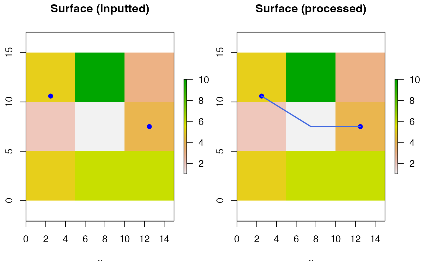 #> ... Calculating Euclidean distance(s)...
#> ... Using method = 'gdistance'...
#> ... ... Defining 'ease' matrix...
#> ... ... Implementing Dijkstra's algorithm to compute least-cost distance(s)...
#> ... ... Implementing Dijkstra's algorithm to compute least-cost path(s)...
#> ... flapper::lcp_over_surface() call completed (@ 2023-08-29 15:44:02) after ~0 minutes.
# As above, paths are stored in path_lcp and distances in dist_lcp
out1$path_lcp
#> $cells
#> path_id path origin destination cell
#> 1 1 1-6 1 6 1
#> 2 1 1-6 1 6 5
#> 3 1 1-6 1 6 6
#>
#> $SpatialLines
#> $SpatialLines$`1`
#> class : SpatialLines
#> features : 1
#> extent : 2.5, 12.5, 7.5, 12.5 (xmin, xmax, ymin, ymax)
#> crs : NA
#>
#>
#> $coordinates
#> $coordinates$`1`
#> x y
#> [1,] 2.5 12.5
#> [2,] 7.5 7.5
#> [3,] 12.5 7.5
#>
#>
# For method = "gdistance", paths between pairs of coordinates are computed
# ... by repeated calls to gdistance::shortestPath(), for each pair of coordinates
# ... in the following list of arguments:
out1$gdistance_param$shortestPath_param
#> $x
#> class : TransitionLayer
#> dimensions : 3, 3, 9 (nrow, ncol, ncell)
#> resolution : 5, 5 (x, y)
#> extent : 0, 15, 0, 15 (xmin, xmax, ymin, ymax)
#> crs : +proj=utm +zone=29 +datum=WGS84 +units=m +no_defs
#> values : conductance
#> matrix class: dsCMatrix
#>
#> $fromCoords
#> x y
#> [1,] 2.5 12.5
#>
#> $toCoords
#> x y
#> [1,] 12.5 7.5
#>
#### Example (11): Parallelisation proceeds as described above via
# ... use_all_cores or cl arguments. For cppRouting, parallelisation
# ... is only implemented for distance calculations (so not if goal = 2),
# ... while parallelisation is implemented for both distance and shortest
# ... paths for method = "gdistance"
out1 <- lcp_over_surface(
origin = rxy[1, , drop = FALSE],
destination = rxy[6, , drop = FALSE],
surface = r,
goal = 3,
use_all_cores = TRUE
)
#> flapper::lcp_over_surface() called (@ 2023-08-29 15:44:02)...
#> ... Checking user inputs...
#> ... Defining cost matrix...
#> Warning: transition function gives negative values
#> ... Calculating Euclidean distance(s)...
#> ... Using method = 'cppRouting'...
#> ... ... Defining nodes, edges and costs to make graph...
#> ... ... Constructing graph object...
#> ... ... Implementing bi algorithm to compute least-cost distance(s)...
#> allcores argument is deprecated since v3.0.
#> Please use RcppParallel::setThreadOptions() to set the number of threads
#> ... Calculating Euclidean distance(s)...
#> ... Using method = 'gdistance'...
#> ... ... Defining 'ease' matrix...
#> ... ... Implementing Dijkstra's algorithm to compute least-cost distance(s)...
#> ... ... Implementing Dijkstra's algorithm to compute least-cost path(s)...
#> ... flapper::lcp_over_surface() call completed (@ 2023-08-29 15:44:02) after ~0 minutes.
# As above, paths are stored in path_lcp and distances in dist_lcp
out1$path_lcp
#> $cells
#> path_id path origin destination cell
#> 1 1 1-6 1 6 1
#> 2 1 1-6 1 6 5
#> 3 1 1-6 1 6 6
#>
#> $SpatialLines
#> $SpatialLines$`1`
#> class : SpatialLines
#> features : 1
#> extent : 2.5, 12.5, 7.5, 12.5 (xmin, xmax, ymin, ymax)
#> crs : NA
#>
#>
#> $coordinates
#> $coordinates$`1`
#> x y
#> [1,] 2.5 12.5
#> [2,] 7.5 7.5
#> [3,] 12.5 7.5
#>
#>
# For method = "gdistance", paths between pairs of coordinates are computed
# ... by repeated calls to gdistance::shortestPath(), for each pair of coordinates
# ... in the following list of arguments:
out1$gdistance_param$shortestPath_param
#> $x
#> class : TransitionLayer
#> dimensions : 3, 3, 9 (nrow, ncol, ncell)
#> resolution : 5, 5 (x, y)
#> extent : 0, 15, 0, 15 (xmin, xmax, ymin, ymax)
#> crs : +proj=utm +zone=29 +datum=WGS84 +units=m +no_defs
#> values : conductance
#> matrix class: dsCMatrix
#>
#> $fromCoords
#> x y
#> [1,] 2.5 12.5
#>
#> $toCoords
#> x y
#> [1,] 12.5 7.5
#>
#### Example (11): Parallelisation proceeds as described above via
# ... use_all_cores or cl arguments. For cppRouting, parallelisation
# ... is only implemented for distance calculations (so not if goal = 2),
# ... while parallelisation is implemented for both distance and shortest
# ... paths for method = "gdistance"
out1 <- lcp_over_surface(
origin = rxy[1, , drop = FALSE],
destination = rxy[6, , drop = FALSE],
surface = r,
goal = 3,
use_all_cores = TRUE
)
#> flapper::lcp_over_surface() called (@ 2023-08-29 15:44:02)...
#> ... Checking user inputs...
#> ... Defining cost matrix...
#> Warning: transition function gives negative values
#> ... Calculating Euclidean distance(s)...
#> ... Using method = 'cppRouting'...
#> ... ... Defining nodes, edges and costs to make graph...
#> ... ... Constructing graph object...
#> ... ... Implementing bi algorithm to compute least-cost distance(s)...
#> allcores argument is deprecated since v3.0.
#> Please use RcppParallel::setThreadOptions() to set the number of threads
 #> ... ... Implementing bi algorithm to compute least-cost paths(s)...
#> ... flapper::lcp_over_surface() call completed (@ 2023-08-29 15:44:02) after ~0 minutes.
out1 <- lcp_over_surface(
origin = rxy[1, , drop = FALSE],
destination = rxy[6, , drop = FALSE],
surface = r,
goal = 2,
method = "gdistance",
cl = parallel::makeCluster(2L)
)
#> flapper::lcp_over_surface() called (@ 2023-08-29 15:44:02)...
#> ... Checking user inputs...
#> ... Defining cost matrix...
#> Warning: transition function gives negative values
#> ... ... Implementing bi algorithm to compute least-cost paths(s)...
#> ... flapper::lcp_over_surface() call completed (@ 2023-08-29 15:44:02) after ~0 minutes.
out1 <- lcp_over_surface(
origin = rxy[1, , drop = FALSE],
destination = rxy[6, , drop = FALSE],
surface = r,
goal = 2,
method = "gdistance",
cl = parallel::makeCluster(2L)
)
#> flapper::lcp_over_surface() called (@ 2023-08-29 15:44:02)...
#> ... Checking user inputs...
#> ... Defining cost matrix...
#> Warning: transition function gives negative values
 #> ... Using method = 'gdistance'...
#> ... ... Defining 'ease' matrix...
#> ... ... Implementing Dijkstra's algorithm to compute least-cost path(s)...
#> ... flapper::lcp_over_surface() call completed (@ 2023-08-29 15:44:08) after ~0.1 minutes.
out1 <- lcp_over_surface(
origin = rxy[1, , drop = FALSE],
destination = rxy[6, , drop = FALSE],
surface = r,
goal = 3,
method = "gdistance",
cl = parallel::makeCluster(2L)
)
#> flapper::lcp_over_surface() called (@ 2023-08-29 15:44:08)...
#> ... Checking user inputs...
#> ... Defining cost matrix...
#> Warning: transition function gives negative values
#> ... Calculating Euclidean distance(s)...
#> ... Using method = 'gdistance'...
#> ... ... Defining 'ease' matrix...
#> ... ... Implementing Dijkstra's algorithm to compute least-cost distance(s)...
#> ... ... Implementing Dijkstra's algorithm to compute least-cost path(s)...
#> ... flapper::lcp_over_surface() call completed (@ 2023-08-29 15:44:13) after ~0.09 minutes.
############################################################################
#### Shortest distances/paths between origin/destination pairs
#### Example (12): Shortest distances/paths computed in sequence:
# cppRouting method
out1 <- lcp_over_surface(
origin = rxy[1:2, , drop = FALSE],
destination = rxy[5:6, , drop = FALSE],
surface = r,
goal = 3
)
#> flapper::lcp_over_surface() called (@ 2023-08-29 15:44:13)...
#> ... Checking user inputs...
#> ... Defining cost matrix...
#> Warning: transition function gives negative values
#> ... Using method = 'gdistance'...
#> ... ... Defining 'ease' matrix...
#> ... ... Implementing Dijkstra's algorithm to compute least-cost path(s)...
#> ... flapper::lcp_over_surface() call completed (@ 2023-08-29 15:44:08) after ~0.1 minutes.
out1 <- lcp_over_surface(
origin = rxy[1, , drop = FALSE],
destination = rxy[6, , drop = FALSE],
surface = r,
goal = 3,
method = "gdistance",
cl = parallel::makeCluster(2L)
)
#> flapper::lcp_over_surface() called (@ 2023-08-29 15:44:08)...
#> ... Checking user inputs...
#> ... Defining cost matrix...
#> Warning: transition function gives negative values
#> ... Calculating Euclidean distance(s)...
#> ... Using method = 'gdistance'...
#> ... ... Defining 'ease' matrix...
#> ... ... Implementing Dijkstra's algorithm to compute least-cost distance(s)...
#> ... ... Implementing Dijkstra's algorithm to compute least-cost path(s)...
#> ... flapper::lcp_over_surface() call completed (@ 2023-08-29 15:44:13) after ~0.09 minutes.
############################################################################
#### Shortest distances/paths between origin/destination pairs
#### Example (12): Shortest distances/paths computed in sequence:
# cppRouting method
out1 <- lcp_over_surface(
origin = rxy[1:2, , drop = FALSE],
destination = rxy[5:6, , drop = FALSE],
surface = r,
goal = 3
)
#> flapper::lcp_over_surface() called (@ 2023-08-29 15:44:13)...
#> ... Checking user inputs...
#> ... Defining cost matrix...
#> Warning: transition function gives negative values
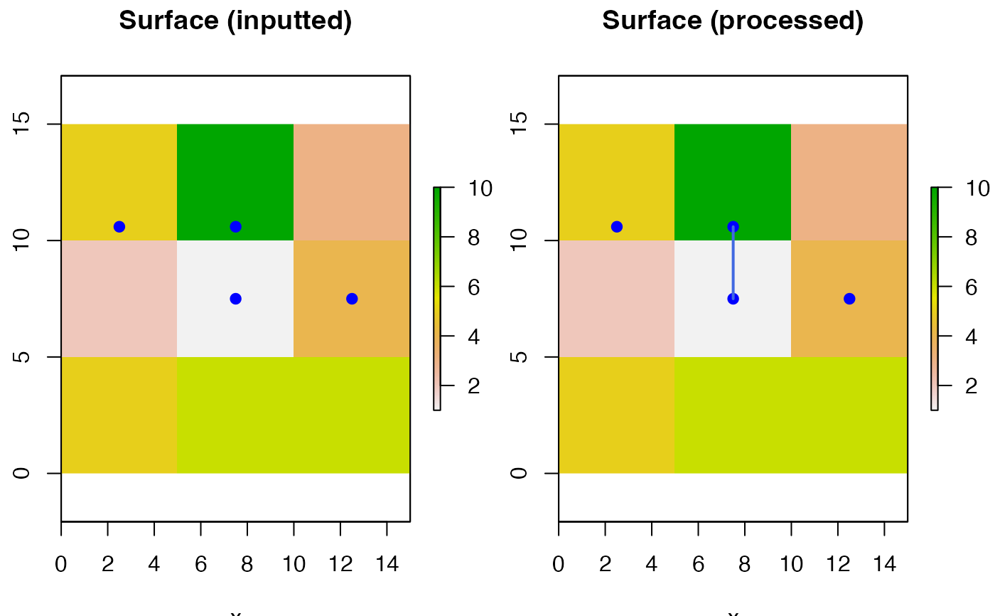 #> ... Calculating Euclidean distance(s)...
#> ... Using method = 'cppRouting'...
#> ... ... Defining nodes, edges and costs to make graph...
#> ... ... Constructing graph object...
#> ... ... Implementing bi algorithm to compute least-cost distance(s)...
#> ... ... Implementing bi algorithm to compute least-cost paths(s)...
#> ... flapper::lcp_over_surface() call completed (@ 2023-08-29 15:44:14) after ~0 minutes.
# gdistance method
out2 <- lcp_over_surface(
origin = rxy[1:2, , drop = FALSE],
destination = rxy[5:6, , drop = FALSE],
surface = r,
goal = 3,
method = "gdistance"
)
#> flapper::lcp_over_surface() called (@ 2023-08-29 15:44:14)...
#> ... Checking user inputs...
#> ... Defining cost matrix...
#> Warning: transition function gives negative values
#> ... Calculating Euclidean distance(s)...
#> ... Using method = 'cppRouting'...
#> ... ... Defining nodes, edges and costs to make graph...
#> ... ... Constructing graph object...
#> ... ... Implementing bi algorithm to compute least-cost distance(s)...
#> ... ... Implementing bi algorithm to compute least-cost paths(s)...
#> ... flapper::lcp_over_surface() call completed (@ 2023-08-29 15:44:14) after ~0 minutes.
# gdistance method
out2 <- lcp_over_surface(
origin = rxy[1:2, , drop = FALSE],
destination = rxy[5:6, , drop = FALSE],
surface = r,
goal = 3,
method = "gdistance"
)
#> flapper::lcp_over_surface() called (@ 2023-08-29 15:44:14)...
#> ... Checking user inputs...
#> ... Defining cost matrix...
#> Warning: transition function gives negative values
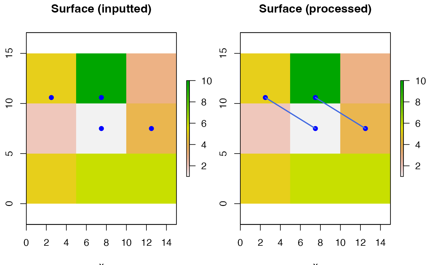 #> ... Calculating Euclidean distance(s)...
#> ... Using method = 'gdistance'...
#> ... ... Defining 'ease' matrix...
#> ... ... Implementing Dijkstra's algorithm to compute least-cost distance(s)...
#> ... ... Implementing Dijkstra's algorithm to compute least-cost path(s)...
#> ... flapper::lcp_over_surface() call completed (@ 2023-08-29 15:44:14) after ~0 minutes.
out1$dist_lcp
#> [1] 8.124038 9.273618
out1$path_lcp
#> $cells
#> path_id path origin destination cell
#> 1 1 2-6 2 6 2
#> 2 1 1-5 1 5 5
#> 3 2 2-6 2 6 6
#>
#> $SpatialLines
#> $SpatialLines$`1`
#> class : SpatialLines
#> features : 1
#> extent : 7.5, 7.5, 7.5, 12.5 (xmin, xmax, ymin, ymax)
#> crs : +proj=utm +zone=29 +datum=WGS84 +units=m +no_defs
#>
#> $SpatialLines$`2`
#> class : SpatialLines
#> features : 1
#> extent : 12.5, 12.5, 7.5, 7.5 (xmin, xmax, ymin, ymax)
#> crs : +proj=utm +zone=29 +datum=WGS84 +units=m +no_defs
#>
#>
#> $coordinates
#> $coordinates$`1`
#> x y
#> [1,] 7.5 12.5
#> [2,] 7.5 7.5
#>
#> $coordinates$`2`
#> x y
#> [1,] 12.5 7.5
#>
#>
out2$dist_lcp
#> [1] 8.124038 9.273618
out2$path_lcp
#> $cells
#> path_id path origin destination cell
#> 1 1 1-5 1 5 1
#> 2 1 1-5 1 5 5
#> 3 2 2-6 2 6 2
#> 4 2 2-6 2 6 6
#>
#> $SpatialLines
#> $SpatialLines$`1`
#> class : SpatialLines
#> features : 1
#> extent : 2.5, 7.5, 7.5, 12.5 (xmin, xmax, ymin, ymax)
#> crs : NA
#>
#> $SpatialLines$`2`
#> class : SpatialLines
#> features : 1
#> extent : 7.5, 12.5, 7.5, 12.5 (xmin, xmax, ymin, ymax)
#> crs : NA
#>
#>
#> $coordinates
#> $coordinates$`1`
#> x y
#> [1,] 2.5 12.5
#> [2,] 7.5 7.5
#>
#> $coordinates$`2`
#> x y
#> [1,] 7.5 12.5
#> [2,] 12.5 7.5
#>
#>
#### Example (13): Shortest distances/paths computed in parallel:
# cppRouting method for goal 3
out1 <- lcp_over_surface(
origin = rxy[1:2, , drop = FALSE],
destination = rxy[5:6, , drop = FALSE],
surface = r,
goal = 3,
use_all_cores = TRUE
)
#> flapper::lcp_over_surface() called (@ 2023-08-29 15:44:14)...
#> ... Checking user inputs...
#> ... Defining cost matrix...
#> Warning: transition function gives negative values
#> ... Calculating Euclidean distance(s)...
#> ... Using method = 'cppRouting'...
#> ... ... Defining nodes, edges and costs to make graph...
#> ... ... Constructing graph object...
#> ... ... Implementing bi algorithm to compute least-cost distance(s)...
#> allcores argument is deprecated since v3.0.
#> Please use RcppParallel::setThreadOptions() to set the number of threads
#> ... Calculating Euclidean distance(s)...
#> ... Using method = 'gdistance'...
#> ... ... Defining 'ease' matrix...
#> ... ... Implementing Dijkstra's algorithm to compute least-cost distance(s)...
#> ... ... Implementing Dijkstra's algorithm to compute least-cost path(s)...
#> ... flapper::lcp_over_surface() call completed (@ 2023-08-29 15:44:14) after ~0 minutes.
out1$dist_lcp
#> [1] 8.124038 9.273618
out1$path_lcp
#> $cells
#> path_id path origin destination cell
#> 1 1 2-6 2 6 2
#> 2 1 1-5 1 5 5
#> 3 2 2-6 2 6 6
#>
#> $SpatialLines
#> $SpatialLines$`1`
#> class : SpatialLines
#> features : 1
#> extent : 7.5, 7.5, 7.5, 12.5 (xmin, xmax, ymin, ymax)
#> crs : +proj=utm +zone=29 +datum=WGS84 +units=m +no_defs
#>
#> $SpatialLines$`2`
#> class : SpatialLines
#> features : 1
#> extent : 12.5, 12.5, 7.5, 7.5 (xmin, xmax, ymin, ymax)
#> crs : +proj=utm +zone=29 +datum=WGS84 +units=m +no_defs
#>
#>
#> $coordinates
#> $coordinates$`1`
#> x y
#> [1,] 7.5 12.5
#> [2,] 7.5 7.5
#>
#> $coordinates$`2`
#> x y
#> [1,] 12.5 7.5
#>
#>
out2$dist_lcp
#> [1] 8.124038 9.273618
out2$path_lcp
#> $cells
#> path_id path origin destination cell
#> 1 1 1-5 1 5 1
#> 2 1 1-5 1 5 5
#> 3 2 2-6 2 6 2
#> 4 2 2-6 2 6 6
#>
#> $SpatialLines
#> $SpatialLines$`1`
#> class : SpatialLines
#> features : 1
#> extent : 2.5, 7.5, 7.5, 12.5 (xmin, xmax, ymin, ymax)
#> crs : NA
#>
#> $SpatialLines$`2`
#> class : SpatialLines
#> features : 1
#> extent : 7.5, 12.5, 7.5, 12.5 (xmin, xmax, ymin, ymax)
#> crs : NA
#>
#>
#> $coordinates
#> $coordinates$`1`
#> x y
#> [1,] 2.5 12.5
#> [2,] 7.5 7.5
#>
#> $coordinates$`2`
#> x y
#> [1,] 7.5 12.5
#> [2,] 12.5 7.5
#>
#>
#### Example (13): Shortest distances/paths computed in parallel:
# cppRouting method for goal 3
out1 <- lcp_over_surface(
origin = rxy[1:2, , drop = FALSE],
destination = rxy[5:6, , drop = FALSE],
surface = r,
goal = 3,
use_all_cores = TRUE
)
#> flapper::lcp_over_surface() called (@ 2023-08-29 15:44:14)...
#> ... Checking user inputs...
#> ... Defining cost matrix...
#> Warning: transition function gives negative values
#> ... Calculating Euclidean distance(s)...
#> ... Using method = 'cppRouting'...
#> ... ... Defining nodes, edges and costs to make graph...
#> ... ... Constructing graph object...
#> ... ... Implementing bi algorithm to compute least-cost distance(s)...
#> allcores argument is deprecated since v3.0.
#> Please use RcppParallel::setThreadOptions() to set the number of threads
 #> ... ... Implementing bi algorithm to compute least-cost paths(s)...
#> ... flapper::lcp_over_surface() call completed (@ 2023-08-29 15:44:14) after ~0 minutes.
# gdistance method for goal 2
out1 <- lcp_over_surface(
origin = rxy[1:2, , drop = FALSE],
destination = rxy[5:6, , drop = FALSE],
surface = r,
goal = 2,
method = "gdistance",
cl = parallel::makeCluster(2L)
)
#> flapper::lcp_over_surface() called (@ 2023-08-29 15:44:14)...
#> ... Checking user inputs...
#> ... Defining cost matrix...
#> Warning: transition function gives negative values
#> ... ... Implementing bi algorithm to compute least-cost paths(s)...
#> ... flapper::lcp_over_surface() call completed (@ 2023-08-29 15:44:14) after ~0 minutes.
# gdistance method for goal 2
out1 <- lcp_over_surface(
origin = rxy[1:2, , drop = FALSE],
destination = rxy[5:6, , drop = FALSE],
surface = r,
goal = 2,
method = "gdistance",
cl = parallel::makeCluster(2L)
)
#> flapper::lcp_over_surface() called (@ 2023-08-29 15:44:14)...
#> ... Checking user inputs...
#> ... Defining cost matrix...
#> Warning: transition function gives negative values
 #> ... Using method = 'gdistance'...
#> ... ... Defining 'ease' matrix...
#> ... ... Implementing Dijkstra's algorithm to compute least-cost path(s)...
#> ... flapper::lcp_over_surface() call completed (@ 2023-08-29 15:44:22) after ~0.13 minutes.
# gdistance method for goal 3
out1 <- lcp_over_surface(
origin = rxy[1:2, , drop = FALSE],
destination = rxy[5:6, , drop = FALSE],
surface = r,
goal = 3,
method = "gdistance",
cl = parallel::makeCluster(2L)
)
#> flapper::lcp_over_surface() called (@ 2023-08-29 15:44:22)...
#> ... Checking user inputs...
#> ... Defining cost matrix...
#> Warning: transition function gives negative values
#> ... Calculating Euclidean distance(s)...
#> ... Using method = 'gdistance'...
#> ... ... Defining 'ease' matrix...
#> ... ... Implementing Dijkstra's algorithm to compute least-cost distance(s)...
#> ... ... Implementing Dijkstra's algorithm to compute least-cost path(s)...
#> ... flapper::lcp_over_surface() call completed (@ 2023-08-29 15:44:34) after ~0.2 minutes.
############################################################################
#### Shortest distances/paths between all origin/destination combinations
#### Example (14) Compute all combinations via combination = "matrix"
# cppRouting goal 3
out1 <- lcp_over_surface(
origin = rxy[1:2, , drop = FALSE],
destination = rxy[5:6, , drop = FALSE],
surface = r,
goal = 3,
cppRouting_algorithm = "phast",
combination = "matrix"
)
#> flapper::lcp_over_surface() called (@ 2023-08-29 15:44:34)...
#> ... Checking user inputs...
#> ... Defining cost matrix...
#> Warning: transition function gives negative values
#> ... Using method = 'gdistance'...
#> ... ... Defining 'ease' matrix...
#> ... ... Implementing Dijkstra's algorithm to compute least-cost path(s)...
#> ... flapper::lcp_over_surface() call completed (@ 2023-08-29 15:44:22) after ~0.13 minutes.
# gdistance method for goal 3
out1 <- lcp_over_surface(
origin = rxy[1:2, , drop = FALSE],
destination = rxy[5:6, , drop = FALSE],
surface = r,
goal = 3,
method = "gdistance",
cl = parallel::makeCluster(2L)
)
#> flapper::lcp_over_surface() called (@ 2023-08-29 15:44:22)...
#> ... Checking user inputs...
#> ... Defining cost matrix...
#> Warning: transition function gives negative values
#> ... Calculating Euclidean distance(s)...
#> ... Using method = 'gdistance'...
#> ... ... Defining 'ease' matrix...
#> ... ... Implementing Dijkstra's algorithm to compute least-cost distance(s)...
#> ... ... Implementing Dijkstra's algorithm to compute least-cost path(s)...
#> ... flapper::lcp_over_surface() call completed (@ 2023-08-29 15:44:34) after ~0.2 minutes.
############################################################################
#### Shortest distances/paths between all origin/destination combinations
#### Example (14) Compute all combinations via combination = "matrix"
# cppRouting goal 3
out1 <- lcp_over_surface(
origin = rxy[1:2, , drop = FALSE],
destination = rxy[5:6, , drop = FALSE],
surface = r,
goal = 3,
cppRouting_algorithm = "phast",
combination = "matrix"
)
#> flapper::lcp_over_surface() called (@ 2023-08-29 15:44:34)...
#> ... Checking user inputs...
#> ... Defining cost matrix...
#> Warning: transition function gives negative values
 #> ... Calculating Euclidean distance(s)...
#> ... Using method = 'cppRouting'...
#> ... ... Defining nodes, edges and costs to make graph...
#> ... ... Constructing graph object...
#> ... ... Implementing phast algorithm to compute least-cost distance(s)...
#> ... .... Implementing Dijkstra's algorithm recursively to compute least-cost paths(s)...
#> ... flapper::lcp_over_surface() call completed (@ 2023-08-29 15:44:34) after ~0 minutes.
out1$dist_euclid
#> 5 6
#> 1 7.071068 11.180340
#> 2 5.000000 7.071068
out1$dist_lcp
#> 5 6
#> 1 8.124038 13.954990
#> 2 10.295630 9.273618
out1$path_lcp
#> $cells
#> path_id path origin destination cell
#> 1 1 1-6 1 6 5
#> 2 1 1-6 1 6 1
#> 3 1 1-5 1 5 5
#> 4 2 2-5 2 5 2
#> 5 2 1-6 1 6 6
#> 6 3 2-6 2 6 2
#> 7 3 2-5 2 5 5
#> 8 4 2-6 2 6 6
#>
#> $SpatialLines
#> $SpatialLines$`1`
#> class : SpatialLines
#> features : 1
#> extent : 2.5, 7.5, 7.5, 12.5 (xmin, xmax, ymin, ymax)
#> crs : +proj=utm +zone=29 +datum=WGS84 +units=m +no_defs
#>
#> $SpatialLines$`2`
#> class : SpatialLines
#> features : 1
#> extent : 7.5, 12.5, 7.5, 12.5 (xmin, xmax, ymin, ymax)
#> crs : +proj=utm +zone=29 +datum=WGS84 +units=m +no_defs
#>
#> $SpatialLines$`3`
#> class : SpatialLines
#> features : 1
#> extent : 7.5, 7.5, 7.5, 12.5 (xmin, xmax, ymin, ymax)
#> crs : +proj=utm +zone=29 +datum=WGS84 +units=m +no_defs
#>
#> $SpatialLines$`4`
#> class : SpatialLines
#> features : 1
#> extent : 12.5, 12.5, 7.5, 7.5 (xmin, xmax, ymin, ymax)
#> crs : +proj=utm +zone=29 +datum=WGS84 +units=m +no_defs
#>
#>
#> $coordinates
#> $coordinates$`1`
#> x y
#> [1,] 7.5 7.5
#> [2,] 2.5 12.5
#> [3,] 7.5 7.5
#>
#> $coordinates$`2`
#> x y
#> [1,] 7.5 12.5
#> [2,] 12.5 7.5
#>
#> $coordinates$`3`
#> x y
#> [1,] 7.5 12.5
#> [2,] 7.5 7.5
#>
#> $coordinates$`4`
#> x y
#> [1,] 12.5 7.5
#>
#>
# cppRouting goal 3 parallelised
out1 <- lcp_over_surface(
origin = rxy[1:2, , drop = FALSE],
destination = rxy[5:6, , drop = FALSE],
surface = r,
goal = 3,
combination = "matrix",
cppRouting_algorithm = "phast",
use_all_cores = TRUE
)
#> flapper::lcp_over_surface() called (@ 2023-08-29 15:44:34)...
#> ... Checking user inputs...
#> ... Defining cost matrix...
#> Warning: transition function gives negative values
#> ... Calculating Euclidean distance(s)...
#> ... Using method = 'cppRouting'...
#> ... ... Defining nodes, edges and costs to make graph...
#> ... ... Constructing graph object...
#> ... ... Implementing phast algorithm to compute least-cost distance(s)...
#> allcores argument is deprecated since v3.0.
#> Please use RcppParallel::setThreadOptions() to set the number of threads
#> ... .... Implementing Dijkstra's algorithm recursively to compute least-cost paths(s)...
#> ... flapper::lcp_over_surface() call completed (@ 2023-08-29 15:44:34) after ~0 minutes.
# gdistance goal 3
out1 <- lcp_over_surface(
origin = rxy[1:2, , drop = FALSE],
destination = rxy[5:6, , drop = FALSE],
surface = r,
goal = 3,
method = "gdistance",
combination = "matrix",
cl = parallel::makeCluster(2L)
)
#> flapper::lcp_over_surface() called (@ 2023-08-29 15:44:34)...
#> ... Checking user inputs...
#> ... Defining cost matrix...
#> Warning: transition function gives negative values
#> ... Calculating Euclidean distance(s)...
#> ... Using method = 'cppRouting'...
#> ... ... Defining nodes, edges and costs to make graph...
#> ... ... Constructing graph object...
#> ... ... Implementing phast algorithm to compute least-cost distance(s)...
#> ... .... Implementing Dijkstra's algorithm recursively to compute least-cost paths(s)...
#> ... flapper::lcp_over_surface() call completed (@ 2023-08-29 15:44:34) after ~0 minutes.
out1$dist_euclid
#> 5 6
#> 1 7.071068 11.180340
#> 2 5.000000 7.071068
out1$dist_lcp
#> 5 6
#> 1 8.124038 13.954990
#> 2 10.295630 9.273618
out1$path_lcp
#> $cells
#> path_id path origin destination cell
#> 1 1 1-6 1 6 5
#> 2 1 1-6 1 6 1
#> 3 1 1-5 1 5 5
#> 4 2 2-5 2 5 2
#> 5 2 1-6 1 6 6
#> 6 3 2-6 2 6 2
#> 7 3 2-5 2 5 5
#> 8 4 2-6 2 6 6
#>
#> $SpatialLines
#> $SpatialLines$`1`
#> class : SpatialLines
#> features : 1
#> extent : 2.5, 7.5, 7.5, 12.5 (xmin, xmax, ymin, ymax)
#> crs : +proj=utm +zone=29 +datum=WGS84 +units=m +no_defs
#>
#> $SpatialLines$`2`
#> class : SpatialLines
#> features : 1
#> extent : 7.5, 12.5, 7.5, 12.5 (xmin, xmax, ymin, ymax)
#> crs : +proj=utm +zone=29 +datum=WGS84 +units=m +no_defs
#>
#> $SpatialLines$`3`
#> class : SpatialLines
#> features : 1
#> extent : 7.5, 7.5, 7.5, 12.5 (xmin, xmax, ymin, ymax)
#> crs : +proj=utm +zone=29 +datum=WGS84 +units=m +no_defs
#>
#> $SpatialLines$`4`
#> class : SpatialLines
#> features : 1
#> extent : 12.5, 12.5, 7.5, 7.5 (xmin, xmax, ymin, ymax)
#> crs : +proj=utm +zone=29 +datum=WGS84 +units=m +no_defs
#>
#>
#> $coordinates
#> $coordinates$`1`
#> x y
#> [1,] 7.5 7.5
#> [2,] 2.5 12.5
#> [3,] 7.5 7.5
#>
#> $coordinates$`2`
#> x y
#> [1,] 7.5 12.5
#> [2,] 12.5 7.5
#>
#> $coordinates$`3`
#> x y
#> [1,] 7.5 12.5
#> [2,] 7.5 7.5
#>
#> $coordinates$`4`
#> x y
#> [1,] 12.5 7.5
#>
#>
# cppRouting goal 3 parallelised
out1 <- lcp_over_surface(
origin = rxy[1:2, , drop = FALSE],
destination = rxy[5:6, , drop = FALSE],
surface = r,
goal = 3,
combination = "matrix",
cppRouting_algorithm = "phast",
use_all_cores = TRUE
)
#> flapper::lcp_over_surface() called (@ 2023-08-29 15:44:34)...
#> ... Checking user inputs...
#> ... Defining cost matrix...
#> Warning: transition function gives negative values
#> ... Calculating Euclidean distance(s)...
#> ... Using method = 'cppRouting'...
#> ... ... Defining nodes, edges and costs to make graph...
#> ... ... Constructing graph object...
#> ... ... Implementing phast algorithm to compute least-cost distance(s)...
#> allcores argument is deprecated since v3.0.
#> Please use RcppParallel::setThreadOptions() to set the number of threads
#> ... .... Implementing Dijkstra's algorithm recursively to compute least-cost paths(s)...
#> ... flapper::lcp_over_surface() call completed (@ 2023-08-29 15:44:34) after ~0 minutes.
# gdistance goal 3
out1 <- lcp_over_surface(
origin = rxy[1:2, , drop = FALSE],
destination = rxy[5:6, , drop = FALSE],
surface = r,
goal = 3,
method = "gdistance",
combination = "matrix",
cl = parallel::makeCluster(2L)
)
#> flapper::lcp_over_surface() called (@ 2023-08-29 15:44:34)...
#> ... Checking user inputs...
#> ... Defining cost matrix...
#> Warning: transition function gives negative values
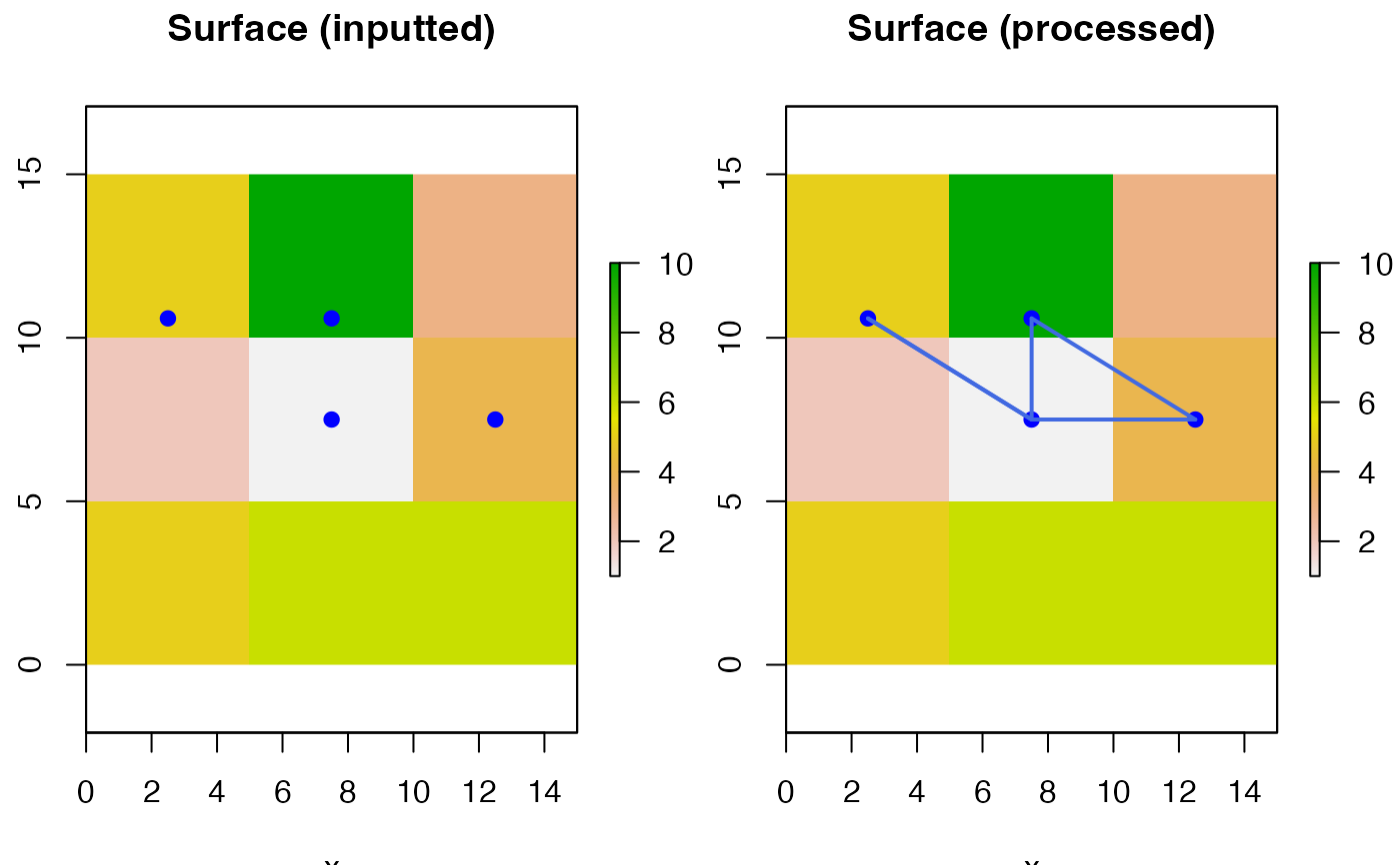 #> ... Calculating Euclidean distance(s)...
#> ... Using method = 'gdistance'...
#> ... ... Defining 'ease' matrix...
#> ... ... Implementing Dijkstra's algorithm to compute least-cost distance(s)...
#> ... ... Implementing Dijkstra's algorithm to compute least-cost path(s)...
#> ... flapper::lcp_over_surface() call completed (@ 2023-08-29 15:44:44) after ~0.16 minutes.
out1$dist_euclid
#> 5 6
#> 1 7.071068 11.180340
#> 2 5.000000 7.071068
out1$dist_lcp
#> 5 6
#> 1 8.124038 13.954990
#> 2 10.295630 9.273618
out1$path_lcp
#> $cells
#> path_id path origin destination cell
#> 1 1 1-5 1 5 1
#> 2 1 1-5 1 5 5
#> 3 2 2-5 2 5 2
#> 4 2 2-5 2 5 5
#> 5 3 1-6 1 6 1
#> 6 3 1-6 1 6 5
#> 7 3 1-6 1 6 6
#> 8 4 2-6 2 6 2
#> 9 4 2-6 2 6 6
#>
#> $SpatialLines
#> $SpatialLines$`1`
#> class : SpatialLines
#> features : 1
#> extent : 2.5, 7.5, 7.5, 12.5 (xmin, xmax, ymin, ymax)
#> crs : NA
#>
#> $SpatialLines$`2`
#> class : SpatialLines
#> features : 1
#> extent : 7.5, 7.5, 7.5, 12.5 (xmin, xmax, ymin, ymax)
#> crs : NA
#>
#> $SpatialLines$`3`
#> class : SpatialLines
#> features : 1
#> extent : 2.5, 12.5, 7.5, 12.5 (xmin, xmax, ymin, ymax)
#> crs : NA
#>
#> $SpatialLines$`4`
#> class : SpatialLines
#> features : 1
#> extent : 7.5, 12.5, 7.5, 12.5 (xmin, xmax, ymin, ymax)
#> crs : NA
#>
#>
#> $coordinates
#> $coordinates$`1`
#> x y
#> [1,] 2.5 12.5
#> [2,] 7.5 7.5
#>
#> $coordinates$`2`
#> x y
#> [1,] 7.5 12.5
#> [2,] 7.5 7.5
#>
#> $coordinates$`3`
#> x y
#> [1,] 2.5 12.5
#> [2,] 7.5 7.5
#> [3,] 12.5 7.5
#>
#> $coordinates$`4`
#> x y
#> [1,] 7.5 12.5
#> [2,] 12.5 7.5
#>
#>
#### Example (15): Real world example with multiple origins/destinations
## Zoom in on an area of interest
ext <- raster::extent(715000, 720000, 6250000, 6260000)
dat_gebco_utm_planar_zoom <- raster::crop(dat_gebco_utm_planar, ext)
## Define example origins/destinations
# Define available coordinates
dat_gebco_utm_planar_zoom_xy <- raster::coordinates(dat_gebco_utm_planar_zoom)
# Sample random origins
set.seed(2019)
index <- sample(1:nrow(dat_gebco_utm_planar_zoom_xy), 2)
origin <- dat_gebco_utm_planar_zoom_xy[index, ]
# Sample random destinations
set.seed(2020)
index <- sample(1:nrow(dat_gebco_utm_planar_zoom_xy), 3)
destination <- dat_gebco_utm_planar_zoom_xy[index, ]
# Implement algorithm
out_gebco1 <- lcp_over_surface(
origin = origin,
destination = destination,
surface = dat_gebco_utm_planar,
method = "gdistance",
goal = 3,
combination = "matrix"
)
#> flapper::lcp_over_surface() called (@ 2023-08-29 15:44:44)...
#> ... Checking user inputs...
#> ... Defining cost matrix...
#> Warning: transition function gives negative values
#> ... Calculating Euclidean distance(s)...
#> ... Using method = 'gdistance'...
#> ... ... Defining 'ease' matrix...
#> ... ... Implementing Dijkstra's algorithm to compute least-cost distance(s)...
#> ... ... Implementing Dijkstra's algorithm to compute least-cost path(s)...
#> ... flapper::lcp_over_surface() call completed (@ 2023-08-29 15:44:44) after ~0.16 minutes.
out1$dist_euclid
#> 5 6
#> 1 7.071068 11.180340
#> 2 5.000000 7.071068
out1$dist_lcp
#> 5 6
#> 1 8.124038 13.954990
#> 2 10.295630 9.273618
out1$path_lcp
#> $cells
#> path_id path origin destination cell
#> 1 1 1-5 1 5 1
#> 2 1 1-5 1 5 5
#> 3 2 2-5 2 5 2
#> 4 2 2-5 2 5 5
#> 5 3 1-6 1 6 1
#> 6 3 1-6 1 6 5
#> 7 3 1-6 1 6 6
#> 8 4 2-6 2 6 2
#> 9 4 2-6 2 6 6
#>
#> $SpatialLines
#> $SpatialLines$`1`
#> class : SpatialLines
#> features : 1
#> extent : 2.5, 7.5, 7.5, 12.5 (xmin, xmax, ymin, ymax)
#> crs : NA
#>
#> $SpatialLines$`2`
#> class : SpatialLines
#> features : 1
#> extent : 7.5, 7.5, 7.5, 12.5 (xmin, xmax, ymin, ymax)
#> crs : NA
#>
#> $SpatialLines$`3`
#> class : SpatialLines
#> features : 1
#> extent : 2.5, 12.5, 7.5, 12.5 (xmin, xmax, ymin, ymax)
#> crs : NA
#>
#> $SpatialLines$`4`
#> class : SpatialLines
#> features : 1
#> extent : 7.5, 12.5, 7.5, 12.5 (xmin, xmax, ymin, ymax)
#> crs : NA
#>
#>
#> $coordinates
#> $coordinates$`1`
#> x y
#> [1,] 2.5 12.5
#> [2,] 7.5 7.5
#>
#> $coordinates$`2`
#> x y
#> [1,] 7.5 12.5
#> [2,] 7.5 7.5
#>
#> $coordinates$`3`
#> x y
#> [1,] 2.5 12.5
#> [2,] 7.5 7.5
#> [3,] 12.5 7.5
#>
#> $coordinates$`4`
#> x y
#> [1,] 7.5 12.5
#> [2,] 12.5 7.5
#>
#>
#### Example (15): Real world example with multiple origins/destinations
## Zoom in on an area of interest
ext <- raster::extent(715000, 720000, 6250000, 6260000)
dat_gebco_utm_planar_zoom <- raster::crop(dat_gebco_utm_planar, ext)
## Define example origins/destinations
# Define available coordinates
dat_gebco_utm_planar_zoom_xy <- raster::coordinates(dat_gebco_utm_planar_zoom)
# Sample random origins
set.seed(2019)
index <- sample(1:nrow(dat_gebco_utm_planar_zoom_xy), 2)
origin <- dat_gebco_utm_planar_zoom_xy[index, ]
# Sample random destinations
set.seed(2020)
index <- sample(1:nrow(dat_gebco_utm_planar_zoom_xy), 3)
destination <- dat_gebco_utm_planar_zoom_xy[index, ]
# Implement algorithm
out_gebco1 <- lcp_over_surface(
origin = origin,
destination = destination,
surface = dat_gebco_utm_planar,
method = "gdistance",
goal = 3,
combination = "matrix"
)
#> flapper::lcp_over_surface() called (@ 2023-08-29 15:44:44)...
#> ... Checking user inputs...
#> ... Defining cost matrix...
#> Warning: transition function gives negative values
 #> ... Calculating Euclidean distance(s)...
#> ... Using method = 'gdistance'...
#> ... ... Defining 'ease' matrix...
#> ... ... Implementing Dijkstra's algorithm to compute least-cost distance(s)...
#> ... ... Implementing Dijkstra's algorithm to compute least-cost path(s)...
#> ... flapper::lcp_over_surface() call completed (@ 2023-08-29 15:44:44) after ~0.01 minutes.
out_gebco2 <- lcp_over_surface(
origin = origin,
destination = destination,
surface = dat_gebco_utm_planar,
method = "cppRouting",
goal = 3,
combination = "matrix",
cppRouting_algorithm = "phast"
)
#> flapper::lcp_over_surface() called (@ 2023-08-29 15:44:44)...
#> ... Checking user inputs...
#> ... Defining cost matrix...
#> Warning: transition function gives negative values
#> ... Calculating Euclidean distance(s)...
#> ... Using method = 'cppRouting'...
#> ... ... Defining nodes, edges and costs to make graph...
#> ... ... Constructing graph object...
#> ... ... Implementing phast algorithm to compute least-cost distance(s)...
#> ... .... Implementing Dijkstra's algorithm recursively to compute least-cost paths(s)...
#> Warning: number of rows of result is not a multiple of vector length (arg 1)
#> ... Calculating Euclidean distance(s)...
#> ... Using method = 'gdistance'...
#> ... ... Defining 'ease' matrix...
#> ... ... Implementing Dijkstra's algorithm to compute least-cost distance(s)...
#> ... ... Implementing Dijkstra's algorithm to compute least-cost path(s)...
#> ... flapper::lcp_over_surface() call completed (@ 2023-08-29 15:44:44) after ~0.01 minutes.
out_gebco2 <- lcp_over_surface(
origin = origin,
destination = destination,
surface = dat_gebco_utm_planar,
method = "cppRouting",
goal = 3,
combination = "matrix",
cppRouting_algorithm = "phast"
)
#> flapper::lcp_over_surface() called (@ 2023-08-29 15:44:44)...
#> ... Checking user inputs...
#> ... Defining cost matrix...
#> Warning: transition function gives negative values
#> ... Calculating Euclidean distance(s)...
#> ... Using method = 'cppRouting'...
#> ... ... Defining nodes, edges and costs to make graph...
#> ... ... Constructing graph object...
#> ... ... Implementing phast algorithm to compute least-cost distance(s)...
#> ... .... Implementing Dijkstra's algorithm recursively to compute least-cost paths(s)...
#> Warning: number of rows of result is not a multiple of vector length (arg 1)
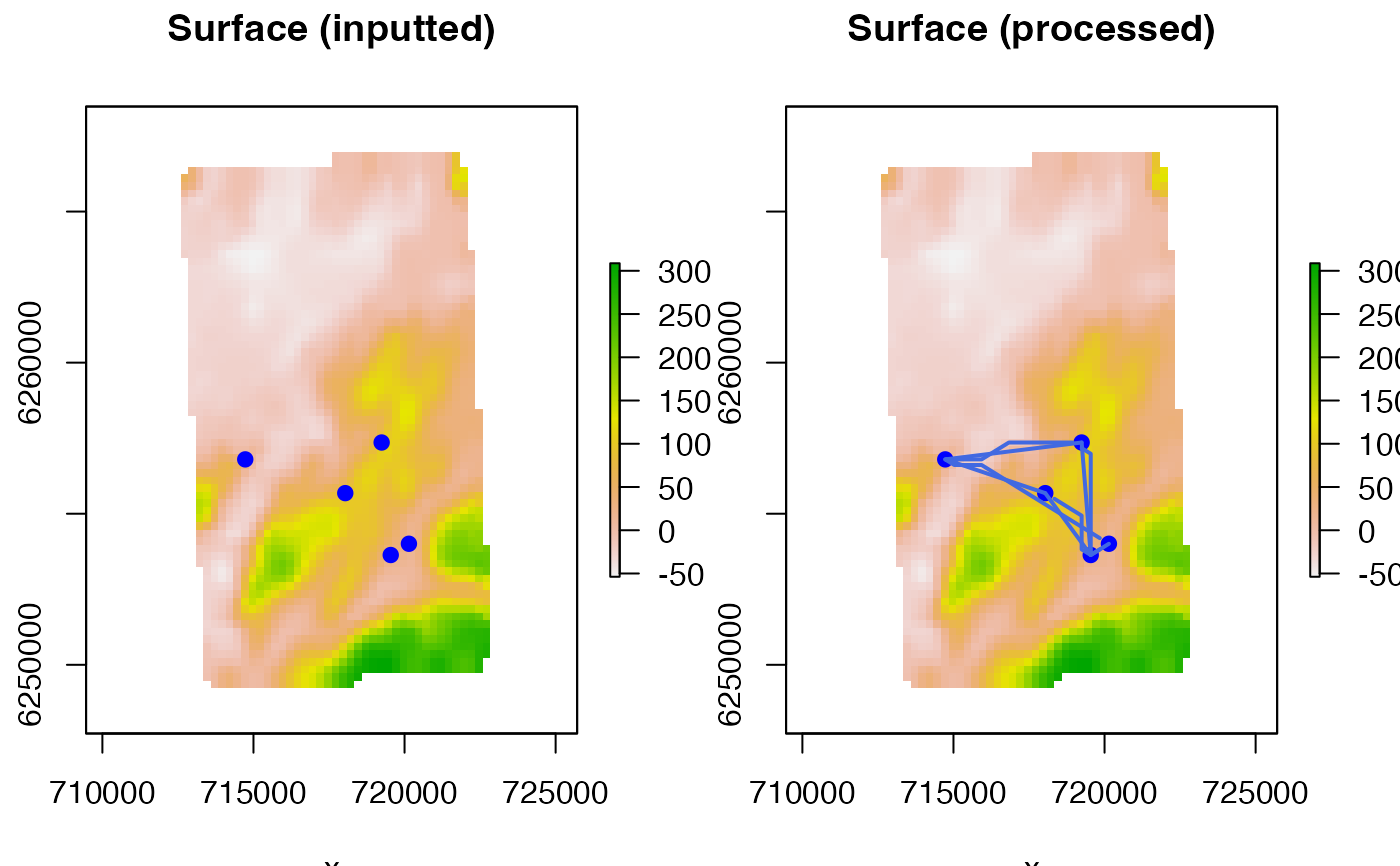 #> ... flapper::lcp_over_surface() call completed (@ 2023-08-29 15:44:45) after ~0.01 minutes.
# The function returns distances between all combinations
out_gebco1$dist_lcp
#> 2945 2463 3438
#> 2610 3375.062 4064.206 6062.3124
#> 3544 3270.267 5106.123 707.1401
out_gebco2$dist_lcp
#> 2945 2463 3438
#> 2610 3375.062 4064.206 6062.3124
#> 3544 3270.267 5106.123 707.1401
# The two outputs are the same (though the ordering of factor levels differs)
str(out_gebco1$path_lcp$cells)
#> 'data.frame': 83 obs. of 5 variables:
#> $ path_id : num 1 1 1 1 1 1 1 1 1 1 ...
#> $ path : Factor w/ 6 levels "2610-2945","3544-2945",..: 1 1 1 1 1 1 1 1 1 1 ...
#> $ origin : int 2610 2610 2610 2610 2610 2610 2610 2610 2610 2610 ...
#> $ destination: int 2945 2945 2945 2945 2945 2945 2945 2945 2945 2945 ...
#> $ cell : int 2610 2665 2666 2667 2668 2723 2778 2833 2834 2835 ...
str(out_gebco2$path_lcp$cells)
#> 'data.frame': 72 obs. of 5 variables:
#> $ path_id : num 1 1 1 1 1 1 1 1 1 1 ...
#> $ path : Factor w/ 6 levels "2610-2945","2610-2463",..: 2 2 2 2 2 2 2 2 2 2 ...
#> $ origin : int 2610 2610 2610 2610 2610 2610 2610 2610 2610 2610 ...
#> $ destination: int 2463 2463 2463 2463 2463 2463 2463 2463 2463 2463 ...
#> $ cell : int 2462 2461 2460 2459 2458 2457 2456 2455 2508 2561 ...
#> ... flapper::lcp_over_surface() call completed (@ 2023-08-29 15:44:45) after ~0.01 minutes.
# The function returns distances between all combinations
out_gebco1$dist_lcp
#> 2945 2463 3438
#> 2610 3375.062 4064.206 6062.3124
#> 3544 3270.267 5106.123 707.1401
out_gebco2$dist_lcp
#> 2945 2463 3438
#> 2610 3375.062 4064.206 6062.3124
#> 3544 3270.267 5106.123 707.1401
# The two outputs are the same (though the ordering of factor levels differs)
str(out_gebco1$path_lcp$cells)
#> 'data.frame': 83 obs. of 5 variables:
#> $ path_id : num 1 1 1 1 1 1 1 1 1 1 ...
#> $ path : Factor w/ 6 levels "2610-2945","3544-2945",..: 1 1 1 1 1 1 1 1 1 1 ...
#> $ origin : int 2610 2610 2610 2610 2610 2610 2610 2610 2610 2610 ...
#> $ destination: int 2945 2945 2945 2945 2945 2945 2945 2945 2945 2945 ...
#> $ cell : int 2610 2665 2666 2667 2668 2723 2778 2833 2834 2835 ...
str(out_gebco2$path_lcp$cells)
#> 'data.frame': 72 obs. of 5 variables:
#> $ path_id : num 1 1 1 1 1 1 1 1 1 1 ...
#> $ path : Factor w/ 6 levels "2610-2945","2610-2463",..: 2 2 2 2 2 2 2 2 2 2 ...
#> $ origin : int 2610 2610 2610 2610 2610 2610 2610 2610 2610 2610 ...
#> $ destination: int 2463 2463 2463 2463 2463 2463 2463 2463 2463 2463 ...
#> $ cell : int 2462 2461 2460 2459 2458 2457 2456 2455 2508 2561 ...