Examine the constant `mobility' assumption of the AC* algorithm(s)

In the simplest and fastest (and only) version of the acoustic-container (AC) and acoustic-container depth-contour (ACDC) algorithms currently implemented by flapper, the rate at which acoustic containers expand and contract depends on a single `mobility' parameter that describes how the set of possible locations for an individual changes through time according to the passive acoustic telemetry data. These changes essentially reflect the maximum horizontal distance that an individual can move in the regularised time steps between sequential detections. However, in some situations, a fixed parameter for horizontal movement may not be well supported. For instance, in cases with archival data (the ACDC algorithm), animals changes dramatically in depth and for which changes in depth are likely to curtail the extent of horizontal movement*. Thus, this function investigates the extent to which the horizontal distance an animal could travel changes through time if the mobility parameter is instead conceptualised as the diagonal distance between sequential depth observations.

acs_setup_mobility(
  depth,
  mobility,
  plot = TRUE,
  add_mobility = list(col = "royalblue", lwd = 2),
  add_rug = list(),
  xlab,
  ...
)

Arguments

depth: A vector of depth observations, whose units match the mobility parameter, to be incorporated into the ACDC algorithm. (Note that the ACDC algorithm may drop depth observations internally depending on their alignment with the acoustic time series and so, ideally, pre-processed time series should be passed to depth to ensure inferences correspond directly to the time series modelled by acdc.) Depth observations should be regularly spaced in time (i.e., represent a time series for a single individual, without gaps).
mobility: A number, in the same units as depth, that defines the maximum horizontal distance that an individual could move in the time period between archival observations (see acs_setup_containers).
plot: A logical variable that defines whether or not to plot the distribution of horizontal distances that the individual could travel, given its depth time series and mobility, as a histogram.
add_mobility: (optional) If plot = TRUE, add_mobility is a named list of arguments, passed to abline, to add the mobility parameter as a vertical line to the histogram as a reference point. add_mobility = NULL suppresses this line.
add_rug: (optional) If plot = TRUE, add_rug is a named list of arguments, passed to rug, to add the estimated distances to the histogram as a rug. add_rug = NULL suppresses this rug.
xlab, ...: Additional arguments, passed to pretty_hist, to customise the histogram.

Value

The function returns a numeric vector of distances and, if plot = TRUE, a histogram of those distances.

Details

The function uses a Pythagorean approximation to estimate the $distance$ that an individual could travel in each time step ($t$), given the maximum horizontal distance that the individual could move ($mobility$) and sequential changes in $depth$, according to the equation:

$$distance_{t + 1} = \sqrt{mobility^2 + (depth_{t + 1} - depth_{t})^2},$$

where $depth_{t + 1}$ for the final ($n^{th}$) observation is defined as $depth_{t = n}$ and thus $distance_{t = n} = mobility$.

*If the horizontal distances that an individual could travel are not very variable, then the benefits of a single mobility parameter are likely to outweigh the costs. On the other hand, substantial variation in the horizontal distances that an individual could travel may suggest that a constant mobility parameter is inappropriate; in this situation, the correct containers could be computed on-the-fly within the ACDC algorithm, but this is not currently implemented. However, the particle filtering algorithms can account for this by the incorporation of movement models within/between acoustic containers.

Author

Edward Lavender

Examples

#### Example (1) Explore mobility for single individual
mob <-
  acs_setup_mobility(
    depth = dat_archival$depth[dat_archival$individual_id == 25],
    mobility = 200
  )


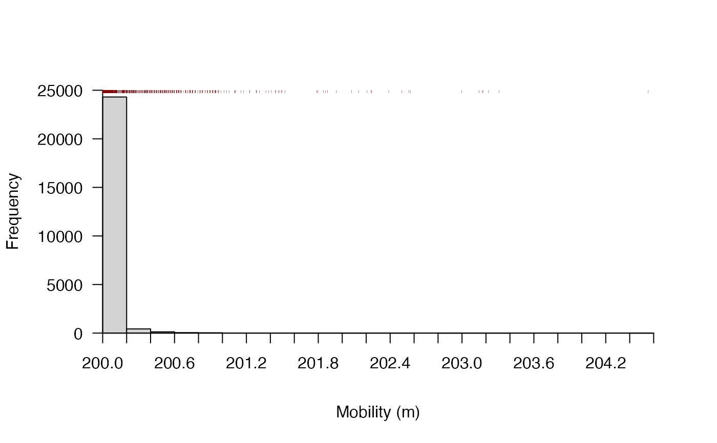
#### Example (2) Customise histogram
# ... suppress plot with plot =  FALSE
# ... suppress add_* lists with NULL or customise
# ... pass args to prettyGraphics::pretty_hist() via ...
mob <-
  acs_setup_mobility(
    depth = dat_archival$depth[dat_archival$individual_id == 25],
    mobility = 200,
    add_mobility = NULL,
    add_rug = list(
      side = 3, pos = 25000,
      col = "darkred", lwd = 0.25, ticksize = 0.01
    ),
    breaks = 25
  )


#### Example (3) Explore mobility for mulitple individuals
pp <- graphics::par(mfrow = c(2, 2))
mob_ls <- lapply(unique(dat_archival$individual_id), function(id) {
  acs_setup_mobility(
    depth = dat_archival$depth[dat_archival$individual_id == id],
    mobility = 200
  )
})
graphics::par(pp)


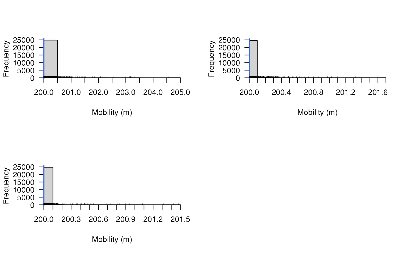#### Results
# For these sample time series, even though the animals change depth
# ... (quite substantially) though time, the sequential changes in depth
# ... are small and the influence on the horizontal distances that they
# ... are assumed to be able to travel in the time gap between archival
# ... observations is so small that a constant mobility parameter
# ... is reasonable without further information (e.g., models of the underlying
# ... behavioural state of the animal). However, it is still likely to be
# ... beneficial to include a movement model to join locations within/
# ... between acoustic containers for some applications via particle filtering.