Pretty histograms

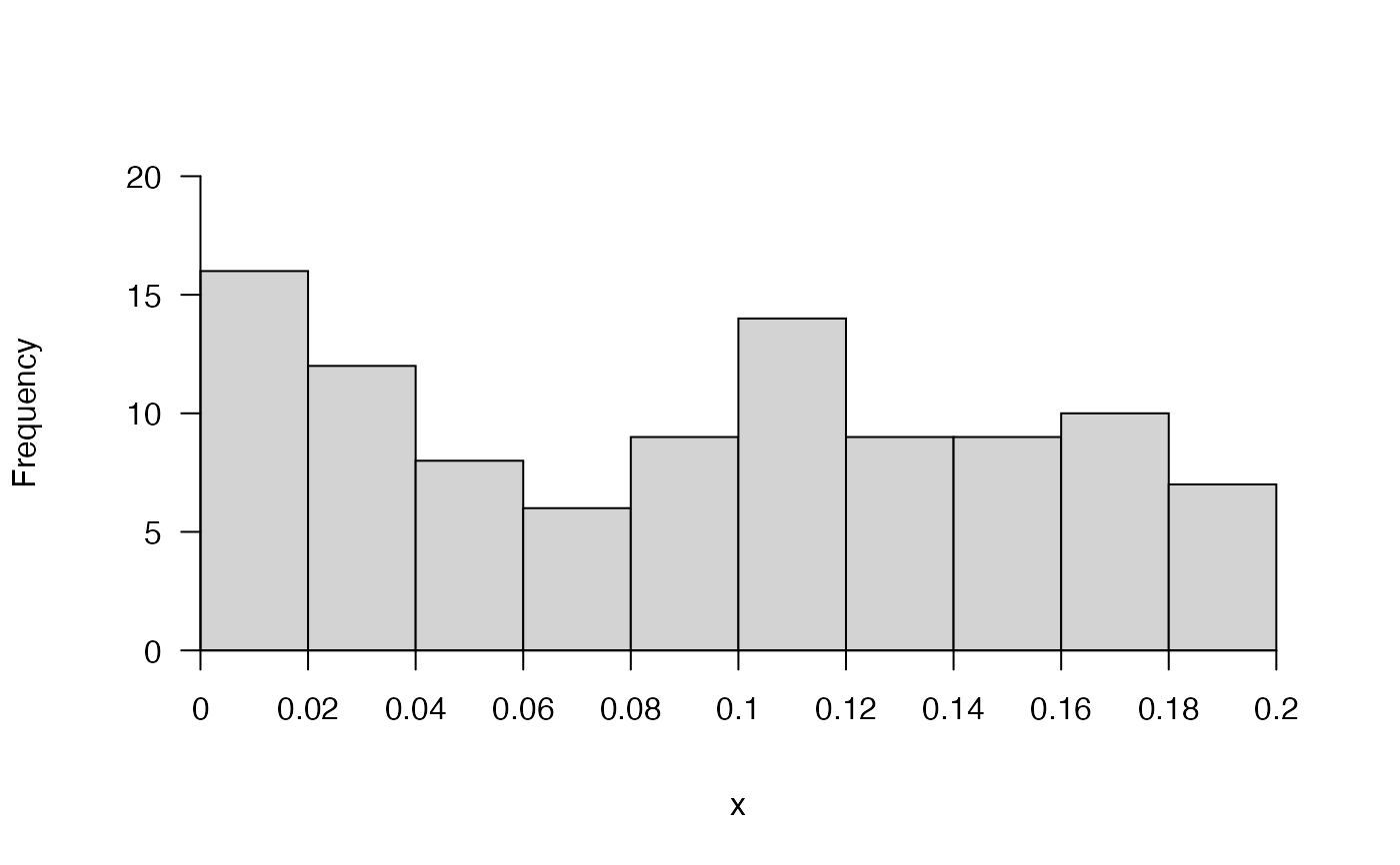
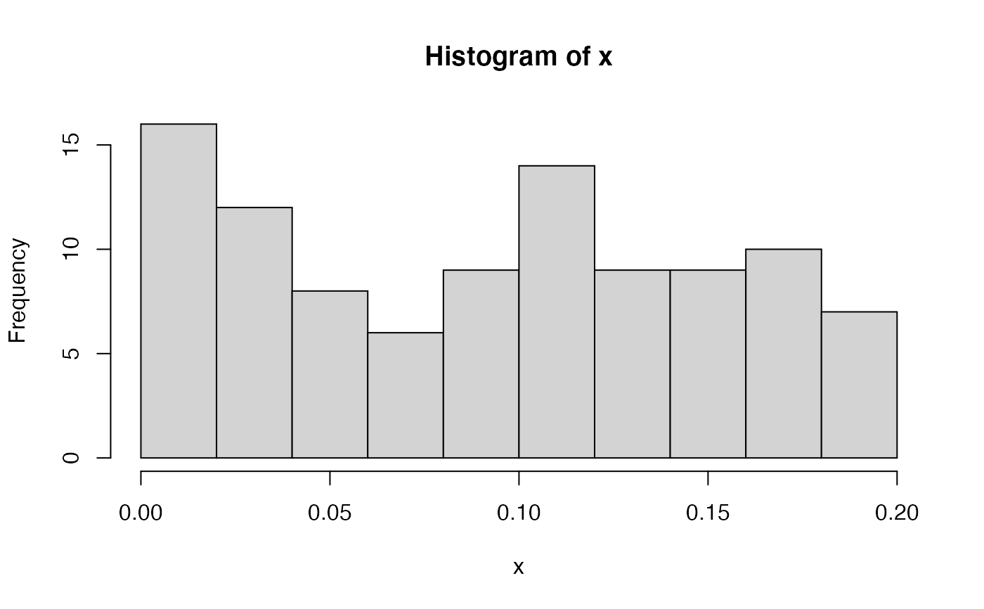
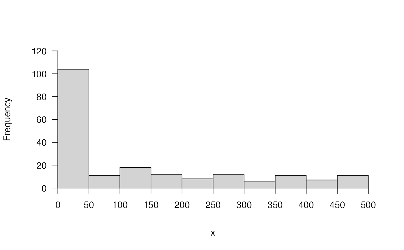
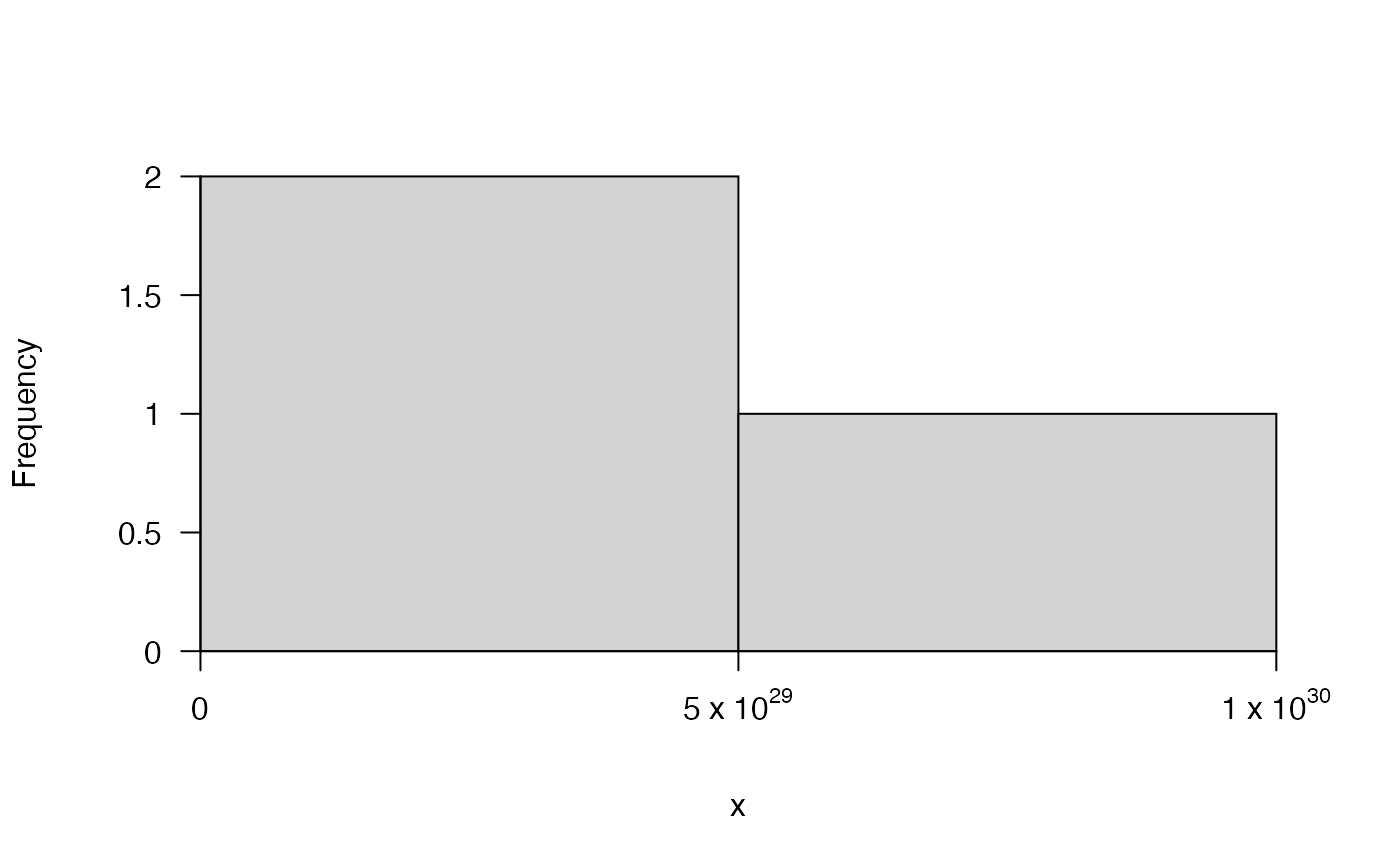
This function makes prettier histograms. Histograms are created using hist with more flexibility for control over the axes. Unlike most functions in prettyGraphics, pretty_hist does not use pretty_axis to draw axes. Instead, by default, the 'breaks' vector computed by hist is used for the x axis, but every xnth value can be selected for inclusion as an axis tick mark. This ensures that axis breaks and tick marks are always aligned. Alternatively, x axis elements can be controlled using xaxis. The default y axis is defined with pretty based on a named list of parameters provided by the user (e.g. including the approximate number of 'pretty' breaks). Alternatively, the y axis can be implemented via yaxis as for the x axis. Axis titles can be added using xlab, ylab or main or via mtext via mtext_args which offers more control.

pretty_hist(
  x,
  freq = TRUE,
  xn = 1,
  ypretty = list(n = 5),
  xaxis = list(),
  yaxis = list(),
  xlim = NULL,
  ylim = NULL,
  xlab = deparse(substitute(x)),
  ylab = ifelse(freq, "Frequency", "Density"),
  main = "",
  control_axis = list(las = TRUE),
  control_sci_notation = list(),
  control_digits = NULL,
  mtext_args = list(),
  ...
)

Arguments

x	A numeric vector for which to create a histogram.
freq	A logical input which defines whether or not to create a histogram of counts or probability densities.
xn	A number which defines the distance between sequential breaks in x retained as x axis labels (i.e., every xnth break is retained as a label; see Description).
ypretty	A named list of parameters, passed to pretty, to create the y axis (see Description).
xaxis	A named list of elements passed to axis to adjust/create the x axis.
yaxis	A named list of elements passed to axis to adjust/create the y axis.
xlim	A vector of two numbers which define the lower and upper x limits of the histogram.
ylim	A vector of two numbers which define the lower and upper y limits of the histogram.
xlab	The x axis label. This can be added via mtext_args for more control.
ylab	The y axis label. This can be added via mtext_args for more control.
main	The plot title. This can be added via mtext_args for more control.
control_axis, control_sci_notation, control_digits	Additional axis control arguments (see pretty_axis).
mtext_args	A named list of arguments passed to mtext to add labels. A nested list is used to control each axis separately.
...	other parameters passed to hist. Arguments that affect the axes should be implemented via xaxis or yaxis; any such arguments passed via ... are silently ignored.

Value

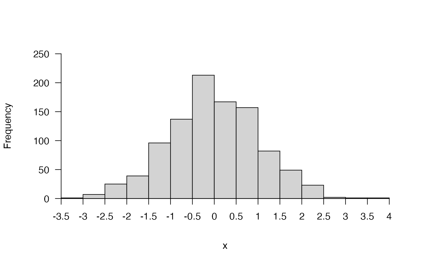
The function returns a pretty histogram.

Author

Edward Lavender

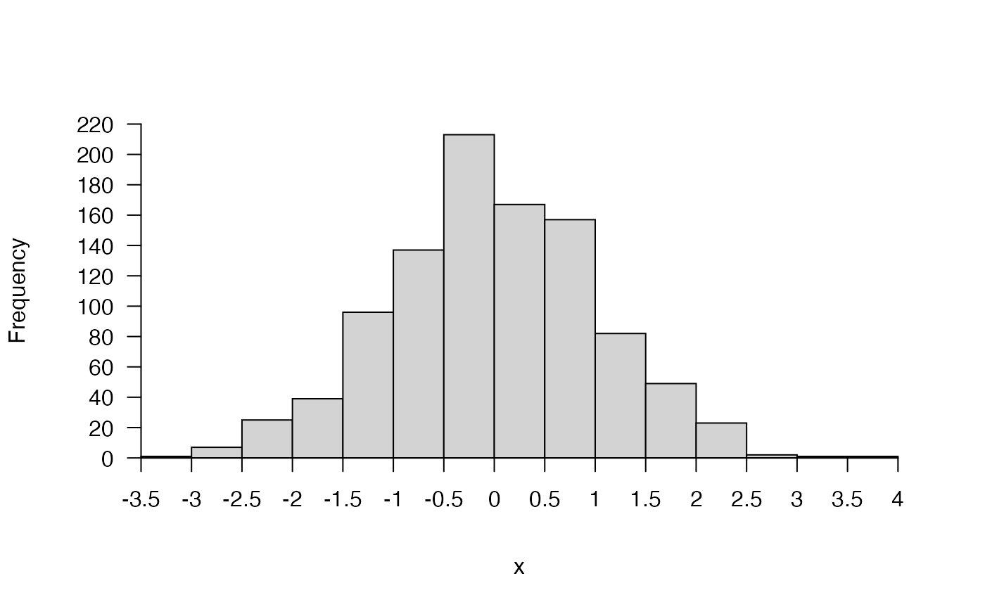
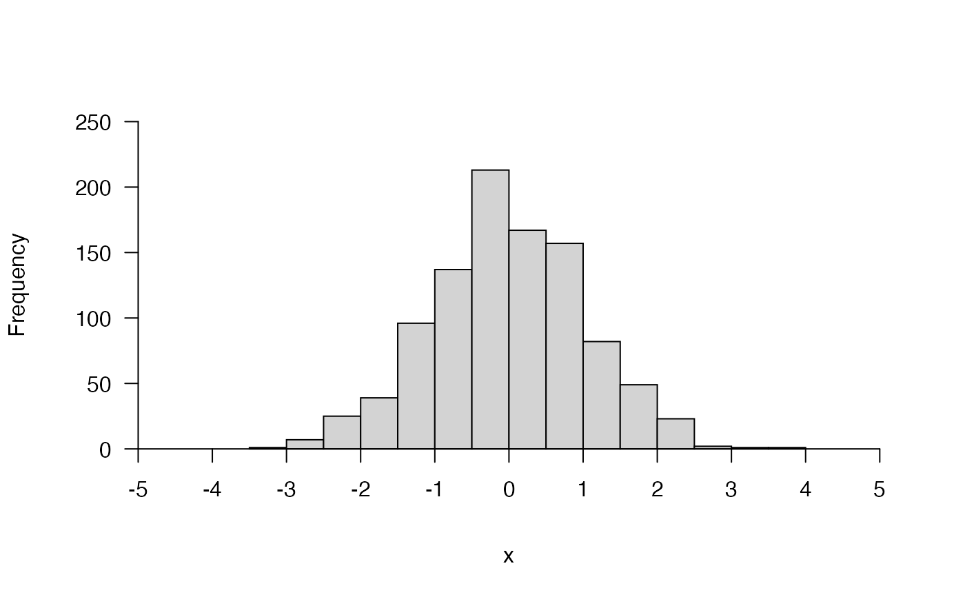
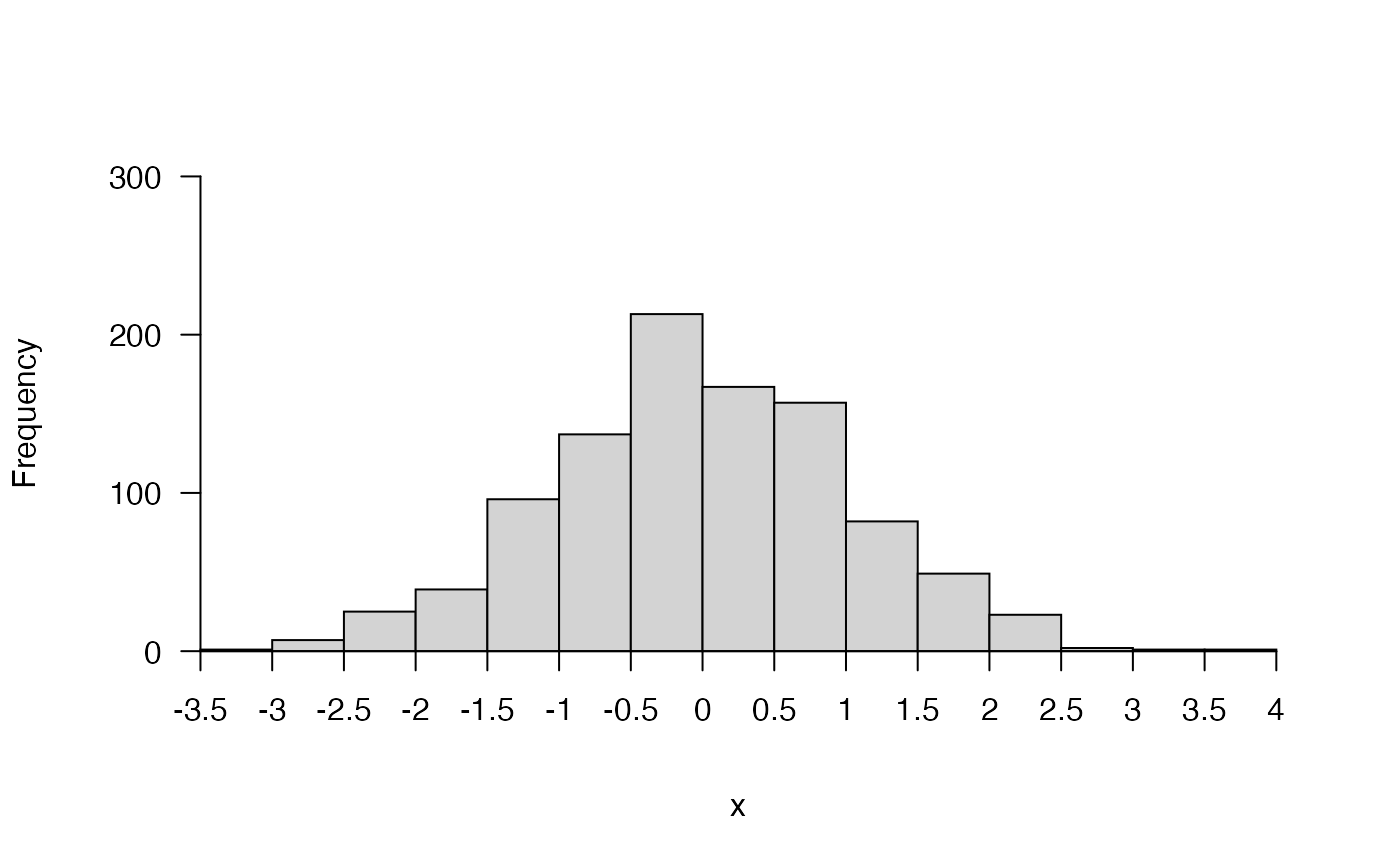
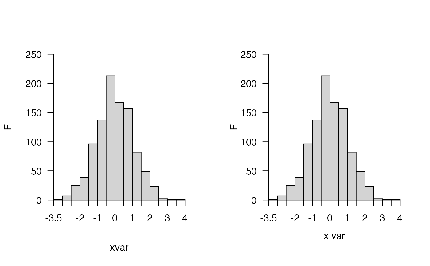
Examples

#### Example (1) The default options
set.seed(1)
x <- rnorm(1000, 0, 1)
pretty_hist(x)

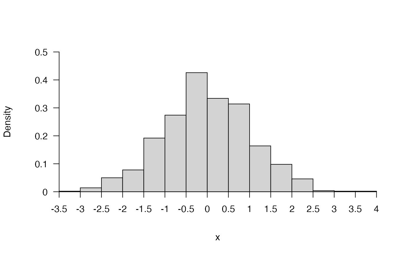
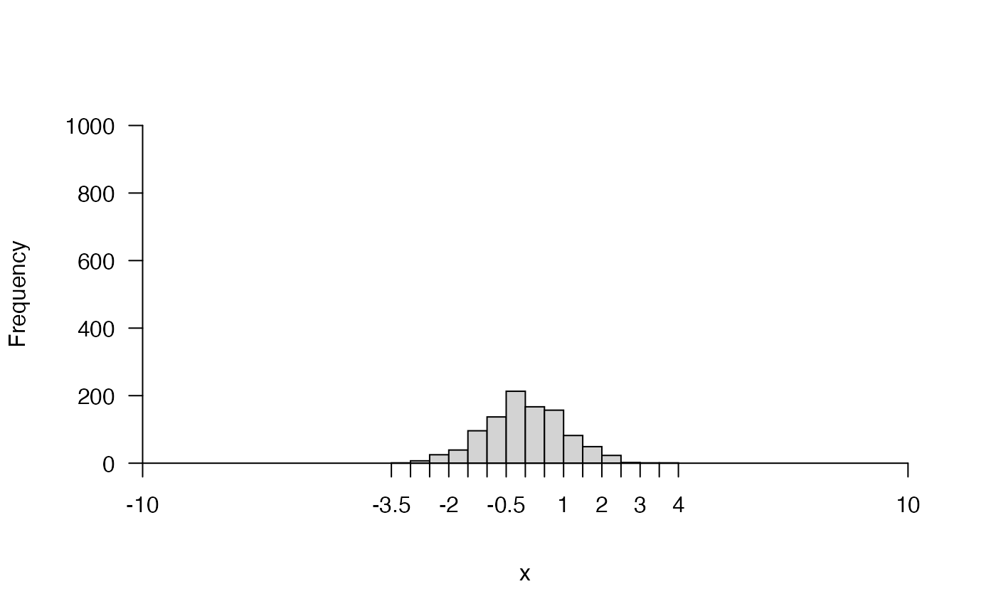
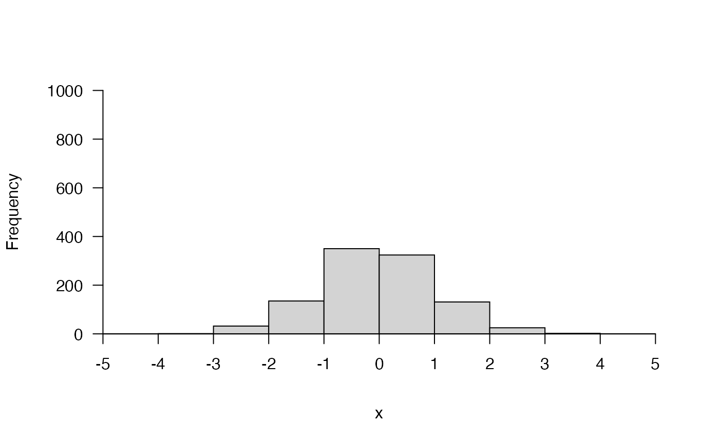
#### Example (2) A density plot
pretty_hist(x, freq = FALSE)

#### Example (3) Axes can be adjusted via xlim, ylim, breaks,
# ... xn, ypretty, or xaxis() and yaxis()
# pp <- par(mfrow = c(1, 6))
pretty_hist(x, xlim = c(-10, 10), ylim = c(0, 1000))
pretty_hist(x, breaks = seq(-5, 5, by = 1), ylim = c(0, 1000))
pretty_hist(x, xn = 2)
pretty_hist(x, ypretty = list(n = 10))
pretty_hist(x, xaxis = list(at = -5:5))
pretty_hist(x, yaxis = list(at = seq(0, 300, by = 100)))
# par(pp)

#### Example (4) Axis labels can be adjusted via mtext() and mtext_args()
pp <- par(mfrow = c(1, 2))
pretty_hist(x, xlab = "xvar", ylab = "F", mtext_args = list())
pretty_hist(x,
            xlab = "", ylab = "",
            mtext_args = list(
               list(side = 1, "x var", line = 2),
               list(side = 2, "F", line = 2)))
par(pp)

#### Example (5) Further  examples
# pp <- par(mfrow = c(4, 2))
# e.g.
x <- c(1.466667, 1.500000)
pretty_hist(x)
hist(x)
# e.g.
x <- runif(100, 0, 0.1987)
pretty_hist(x)
hist(x)
# e.g.
x <- c(runif(100, 0, 0.1987), runif(100, 30, 500))
pretty_hist(x)
hist(x)
# e.g.
x <- c(1e10, 1e20, 1e30)
pretty_hist(x)
hist(x)
# par(pp)

#### Example (6) Some examples with dates and times
## Define some time series data
x <- seq.Date(as.Date("2016-01-01"), as.Date("2017-01-01"), 1)
x <- sample(x, size = 1000, replace = TRUE)
## Set plotting region
pp <- par(mfrow = c(2, 2))
## hist() and pretty_hist() comparison
# Note that for times, hist() displays density by default,
# ... but freq = FALSE is needed for pretty_hist
hist(x, breaks = "months")
pretty_hist(x, breaks = "months", freq = FALSE)
## Usually for time series, you need to be explicit about breaks
# ... for pretty plots:
hist(x,
     breaks = seq(min(x), max(x), by = "months"),
     format = "%d-%m", las = 2)
pretty_hist(x,
            breaks = seq(min(x), max(x), by = "months"),
            xaxis = list(format = "%d-%m", las = 2),
            freq = FALSE
)
par(pp)