The function computes a detection history similarity matrix. For all combinations of individuals, this shows the total number (or percentage) of detections `nearby' in space and time, which can help to elucidate possible interactions among individuals that affect space use (see Details). To compute this matrix, the function pairs detections for each individual with the detections nearest in time for each other individual. The function computes the time (minutes) between paired detection time series, and the distance (m) between the receiver(s) at which paired detections occurred, dropping any detection pairs that are further apart in time or space than user-defined thresholds (which depend on the mobility of the species under investigation). For each combination of individuals, the function returns total number (or percentage) of detections that are closely associated in time and space. For very large combinations of individuals, especially those with long, overlapping time series, the function may take some time to run; therefore, testing the function on a small subset of individuals first is advisable. Parallelisation can be used to improve computation time. Similarity matrices can be visualised with pretty_mat.
make_matrix_cooccurence(
  acoustics_ls,
  thresh_time,
  thresh_dist,
  cl = NULL,
  varlist = NULL,
  output = 1,
  verbose = TRUE
)
Arguments
- acoustics_ls
A list of dataframes, with one element for each individual, which contains each individual's detection time series. Each dataframe must include the following columns: `individual_id', a factor which specifies unique individuals; `timestamp', a POSIXct object which specifies the time of each detection; `receiver_long', the longitude (decimal degrees) of the receiver(s) at the individual was detected; and `receiver_lat', the latitude (decimal degrees) of the receiver(s) at which individual was detected. Each dataframe should be ordered by `individual_id' and then by `timestamp'. Careful ordering of `individual_id' factor levels (e.g. perhaps by population group, then by the number of detections of each individual) can aid visualisation of similarity matrices, in which the order or rows/columns corresponds directly to the order of individuals in
acoustics_ls. Sequential elements inacoustics_lsshould correspond to sequential factor levels for `individual_id', which should be the same across all dataframes.- thresh_time
A number which specifies the time, in minutes, after which detections at nearby receivers are excluded.
- thresh_dist
A number which specifies the (Euclidean) distance between receivers, in metres, beyond which detections are excluded (see Details).
- cl, varlist
(optional)
clis (a) a cluster object frommakeClusteror (b) an integer that defines the number of child processes.varlistis a character vector of variables for export (seecl_export). Exported variables must be located in the global environment. If a cluster is supplied, the connection to the cluster is closed within the function (seecl_stop). For further information, seecl_lapplyandflapper-tips-parallel.- output
A number which specifies the output type. If
output = 1, the function returns a (usually) symmetric similarity matrix in which each number represents the number of detections nearby in space and time for each pair of individuals. Row and column names are assigned from the `individual_id' column inacoustics_lsdataframes. This matrix is usually symmetric, but this is not necessarily the case for data collected from tags which transmit at random intervals around a nominal delay: under this scenario, the tag for a given individual (i) may transmit multiple signals in the space of time that the tag for another individual (j) only releases a single transmission. In this case, the pairing i,j will comprise all unique transmissions for individual i, paired with the nearest observations for individual j, some of which will be duplicate observations. Therefore, this pairing will contain more `shared observations' than the pairing j,i. However, even under random transmission, the matrix will usually be either symmetric or very nearly symmetric, with only small differences between identical pairs. Ifoutput = 2, the function returns a list with the following elements: (1) `mat_sim', the symmetric similarity matrix (see above); `mat_nobs', a matrix with the same dimensions as `mat_sim' which specifies the number of observations for each individual (by row, used to calculate `mat_pc', see later); `mat_pc', a non-symmetric matrix in which each cell represents the percent of observations of the individual in the i'th row that are shared with the individual in the j'th column; and `dat', a nested list, with one element for each individual which comprises a list of dataframes, one for each other individual, each one of which contains the subset of observations that are shared between the two individuals. Each dataframe contains the same columns as in theacoustics_lsdataframes with the following columns added: `pos_in_acc2', `timestamp_acc2', `receiver_lat_acc2' and `receiver_long_acc2', which represent the positions, time stamps and locations of corresponding observations in the second individual's dataframe to the first individual's dataframe, and `difftime_abs' and `dist_btw_receivers' which represent the duration (minutes) and distances (m) between corresponding observations. When there are no shared observations between a pair of individuals, the element simply containsNULL. Note that `mat_pc' is computed by (mat_sim/mat_nobs)*100. The matrix is therefore non-symmetric (if individuals have differing numbers of observations); i.e., mat_pc[i, j] is the percent of individual i's observations that are shared with individual j; while mat_pc[j, i] is the percent of individual j's observations that are shared with individual i. NaN elements are possible in `mat_pc' for levels of the factor `individual_id' without observations.- verbose
A logical input which specifies whether or not to print messages to the console which relay function progress.
Value
The function returns a matrix or a list, depending on the input to output (see above).
Details
Background
Passive acoustic telemetry is widely used to study animal space use, and the possible drivers of spatiotemporal patterns in space use, in aquatic environments. Patterns in space use are widely related to environmental conditions, such as temperature, but the role of interactions among individuals is often more challenging to investigate due to a paucity of data, despite their likely importance. However, discrete detections also contain information on interactions among individuals that may influence space use through their similarities and differences among individuals over time and space.
Implications
Similarities and differences can take different forms with differing ecological implications. For example, for individuals that are frequently detected in similar areas, detections may indicate (a) prolonged associations among individuals, if detections are usually closely associated in time and space (for example, due to parent-offspring relationships, group-living and/or mating); or (b) avoidance and/or territorial-like behaviour if detections, while close in space, are usually at different receivers and/or disjointed in time. Likewise, detection similarities among individuals that are rarely detected, or usually detected at disparate receivers, may reflect important interactions among those individuals at particular times (e.g. mating).
Methods
To explore similarities and differences in patterns of space use, visualisation of detection histories with abacus plots and maps is beneficial. However, with many individuals and large receiver arrays, quantification of the similarities in detections over time and space is challenging. To this end, make_matrix_cooccurence computes a similarity matrix across all individuals, defining the number (or percentage) of detections for each individual that are nearby in time, or space, to detections for each other individual.
Examples
#### Prepare data
# acoustics_ls requires a dataframe with certain columns
# individual_id should be a factor
dat_acoustics$individual_id <- factor(dat_acoustics$individual_id)
# ensure dataframe ordered by individual, then time stamp
dat_acoustics <- dat_acoustics[order(dat_acoustics$individual_id, dat_acoustics$timestamp), ]
# define list of dataframes
acoustics_ls <- split(dat_acoustics, factor(dat_acoustics$individual_id))
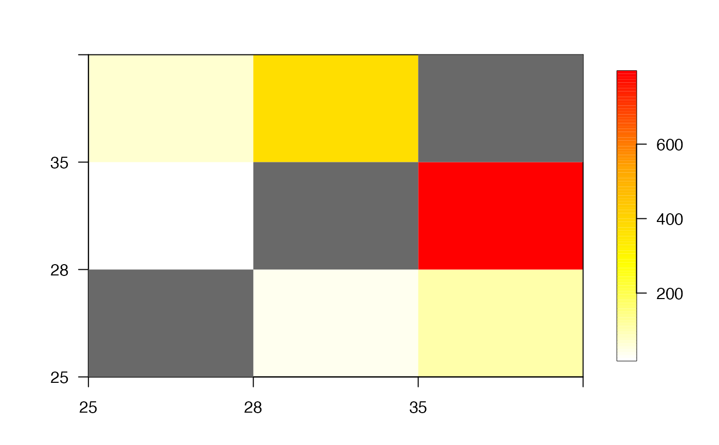
#### Example (1): Compute detection similarity matrix using default options
# mat_sim contains the number of observations shared among individuals
mat_sim <- make_matrix_cooccurence(
acoustics_ls = acoustics_ls,
thresh_time = 90,
thresh_dist = 0
)
#>
#> ===================================================================================
#> Individual ( 25 ) and individual ( 28 ).
#> Matching detection time series...
#> Processing time series by theshold time difference...
#> Computing differences between pairs of receivers...
#> Processing time series by threshold distance...
#>
#> ===================================================================================
#> Individual ( 25 ) and individual ( 35 ).
#> Matching detection time series...
#> Processing time series by theshold time difference...
#> Computing differences between pairs of receivers...
#> Processing time series by threshold distance...
#>
#> ===================================================================================
#> Individual ( 28 ) and individual ( 25 ).
#> Matching detection time series...
#> Processing time series by theshold time difference...
#> Computing differences between pairs of receivers...
#> Processing time series by threshold distance...
#>
#> ===================================================================================
#> Individual ( 28 ) and individual ( 35 ).
#> Matching detection time series...
#> Processing time series by theshold time difference...
#> Computing differences between pairs of receivers...
#> Processing time series by threshold distance...
#>
#> ===================================================================================
#> Individual ( 35 ) and individual ( 25 ).
#> Matching detection time series...
#> Processing time series by theshold time difference...
#> Computing differences between pairs of receivers...
#> Processing time series by threshold distance...
#>
#> ===================================================================================
#> Individual ( 35 ) and individual ( 28 ).
#> Matching detection time series...
#> Processing time series by theshold time difference...
#> Computing differences between pairs of receivers...
#> Processing time series by threshold distance...
prettyGraphics::pretty_mat(mat_sim, col_diag = "dimgrey")
 #### Example (2): Return list of outputs
out_ls <- make_matrix_cooccurence(
acoustics_ls = acoustics_ls,
thresh_time = 90,
thresh_dist = 0,
output = 2
)
#>
#> ===================================================================================
#> Individual ( 25 ) and individual ( 28 ).
#> Matching detection time series...
#> Processing time series by theshold time difference...
#> Computing differences between pairs of receivers...
#> Processing time series by threshold distance...
#>
#> ===================================================================================
#> Individual ( 25 ) and individual ( 35 ).
#> Matching detection time series...
#> Processing time series by theshold time difference...
#> Computing differences between pairs of receivers...
#> Processing time series by threshold distance...
#>
#> ===================================================================================
#> Individual ( 28 ) and individual ( 25 ).
#> Matching detection time series...
#> Processing time series by theshold time difference...
#> Computing differences between pairs of receivers...
#> Processing time series by threshold distance...
#>
#> ===================================================================================
#> Individual ( 28 ) and individual ( 35 ).
#> Matching detection time series...
#> Processing time series by theshold time difference...
#> Computing differences between pairs of receivers...
#> Processing time series by threshold distance...
#>
#> ===================================================================================
#> Individual ( 35 ) and individual ( 25 ).
#> Matching detection time series...
#> Processing time series by theshold time difference...
#> Computing differences between pairs of receivers...
#> Processing time series by threshold distance...
#>
#> ===================================================================================
#> Individual ( 35 ) and individual ( 28 ).
#> Matching detection time series...
#> Processing time series by theshold time difference...
#> Computing differences between pairs of receivers...
#> Processing time series by threshold distance...
names(out_ls)
#> [1] "mat_sim" "mat_nobs" "mat_pc" "dat"
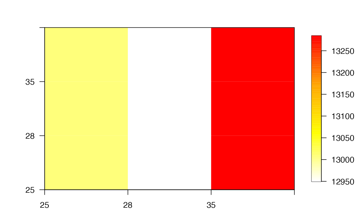
# Examine number of observations for each individual
prettyGraphics::pretty_mat(out_ls$mat_nobs)
#### Example (2): Return list of outputs
out_ls <- make_matrix_cooccurence(
acoustics_ls = acoustics_ls,
thresh_time = 90,
thresh_dist = 0,
output = 2
)
#>
#> ===================================================================================
#> Individual ( 25 ) and individual ( 28 ).
#> Matching detection time series...
#> Processing time series by theshold time difference...
#> Computing differences between pairs of receivers...
#> Processing time series by threshold distance...
#>
#> ===================================================================================
#> Individual ( 25 ) and individual ( 35 ).
#> Matching detection time series...
#> Processing time series by theshold time difference...
#> Computing differences between pairs of receivers...
#> Processing time series by threshold distance...
#>
#> ===================================================================================
#> Individual ( 28 ) and individual ( 25 ).
#> Matching detection time series...
#> Processing time series by theshold time difference...
#> Computing differences between pairs of receivers...
#> Processing time series by threshold distance...
#>
#> ===================================================================================
#> Individual ( 28 ) and individual ( 35 ).
#> Matching detection time series...
#> Processing time series by theshold time difference...
#> Computing differences between pairs of receivers...
#> Processing time series by threshold distance...
#>
#> ===================================================================================
#> Individual ( 35 ) and individual ( 25 ).
#> Matching detection time series...
#> Processing time series by theshold time difference...
#> Computing differences between pairs of receivers...
#> Processing time series by threshold distance...
#>
#> ===================================================================================
#> Individual ( 35 ) and individual ( 28 ).
#> Matching detection time series...
#> Processing time series by theshold time difference...
#> Computing differences between pairs of receivers...
#> Processing time series by threshold distance...
names(out_ls)
#> [1] "mat_sim" "mat_nobs" "mat_pc" "dat"
# Examine number of observations for each individual
prettyGraphics::pretty_mat(out_ls$mat_nobs)
 # Examine % shared detections between individuals
prettyGraphics::pretty_mat(out_ls$mat_pc, col_diag = "dimgrey")
# Examine % shared detections between individuals
prettyGraphics::pretty_mat(out_ls$mat_pc, col_diag = "dimgrey")
 #### Example (3): Turn off messages with verbose = FALSE
out_ls_non_verb <- make_matrix_cooccurence(
acoustics_ls = acoustics_ls,
thresh_time = 90,
thresh_dist = 0,
verbose = FALSE
)
#### Example (4): Implement algorithm in parallel
out_ls_pl <- make_matrix_cooccurence(
acoustics_ls = acoustics_ls,
thresh_time = 90,
thresh_dist = 0,
cl = parallel::makeCluster(2L),
output = 2
)
names(out_ls_pl)
#> [1] "mat_sim" "mat_nobs" "mat_pc" "dat"
#### Example (3): Turn off messages with verbose = FALSE
out_ls_non_verb <- make_matrix_cooccurence(
acoustics_ls = acoustics_ls,
thresh_time = 90,
thresh_dist = 0,
verbose = FALSE
)
#### Example (4): Implement algorithm in parallel
out_ls_pl <- make_matrix_cooccurence(
acoustics_ls = acoustics_ls,
thresh_time = 90,
thresh_dist = 0,
cl = parallel::makeCluster(2L),
output = 2
)
names(out_ls_pl)
#> [1] "mat_sim" "mat_nobs" "mat_pc" "dat"