Plot pretty matrices — pretty_mat • prettyGraphics

This function is a wrapper for image.plot designed to streamline the visualisation of pretty matrices. The function returns a plot which can be customised.

pretty_mat(
  z,
  retain_orientation = FALSE,
  zlim = NULL,
  col = (grDevices::colorRampPalette(c("white", "yellow", "orange", "red")))(100),
  col_diag = NULL,
  grid = NULL,
  add_axes = TRUE,
  xtick_every_n = 1,
  ytick_every_n = xtick_every_n,
  cex.axis = 1,
  las = TRUE,
  xlab = "",
  ylab = "",
  ...
)

Arguments

z	A matrix to be plotted.
retain_orientation	A logical input which defines whether or not the plot should retain the same orientation as the printed matrix. The default is `FALSE`, in which case the underlying plotting function (`image.plot`) rotates the matrix by 90 degrees counter-clockwise in the plot. In contrast, `retain_orientation = TRUE` forces the matrix and the plot to retain the same orientation (see Details).
zlim	A numeric vector of length two which specifies the z axis limits (see `image.plot`),
col	A colour table to use for the image (see `image.plot`).
col_diag	(optional) A colour which, if provided, is used to shade the diagonal of the matrix. This is useful for symmetric square matrices.
grid	(optional) A named list which, if provided, is passed to `add_grid_rect_xy` to draw grid lines around each matrix cell. Arguments `x` and `y` default to the positions of each matrix cell and do not need to be provided. To use `add_grid_rect_xy`'s default graphical options, simply specify `grid = list()`.
add_axes	A logical input which defines whether or not to add axes to the plot. Axes tick marks are given every nth column and every nth row (see below).
xtick_every_n	A numeric input which defines the spacing between sequential tick marks for the x axis. Tick marks are given every `xtick_every_n` (see Details).
ytick_every_n	A numeric input which defines the spacing between sequential tick marks for the other axis. Tick marks are given every `ytick_every_n` (see Details).
cex.axis	A number which specifies the axis font size (see `par`).
las	The style of axis labels (see `par`).
xlab	The x axis label.
ylab	The y axis label.
...	Additional arguments passed to `image.plot`. These should not include `x`, `y`, `xlim`, `ylim` or `axes` which are controlled internally.

Value

The function returns a plot of a matrix with coloured cells.

Details

The limits of the plot are set between (0.5, number of rows + 0.5) and (0.5, number of cols + 0.5). Axes are added by default, but can be suppressed. If available, matrix row/column names are used to define axis labels. Otherwise, an index is used. Axes labels are added every xtick_every_n and ytick_every_n. If retain_orientation is FALSE, the plot is rotated 90 degrees counter-clockwise relative to the input matrix and thus read from the bottom-left to the top-right (like a map), so that matrix columns and corresponding tick mark labels are represented along the y axis whereas matrix rows and corresponding tick mark labels are represented along the x axis. In contrast, if retain_orientation is TRUE, the plot is read from the top-left to bottom-right.

Author

Edward Lavender

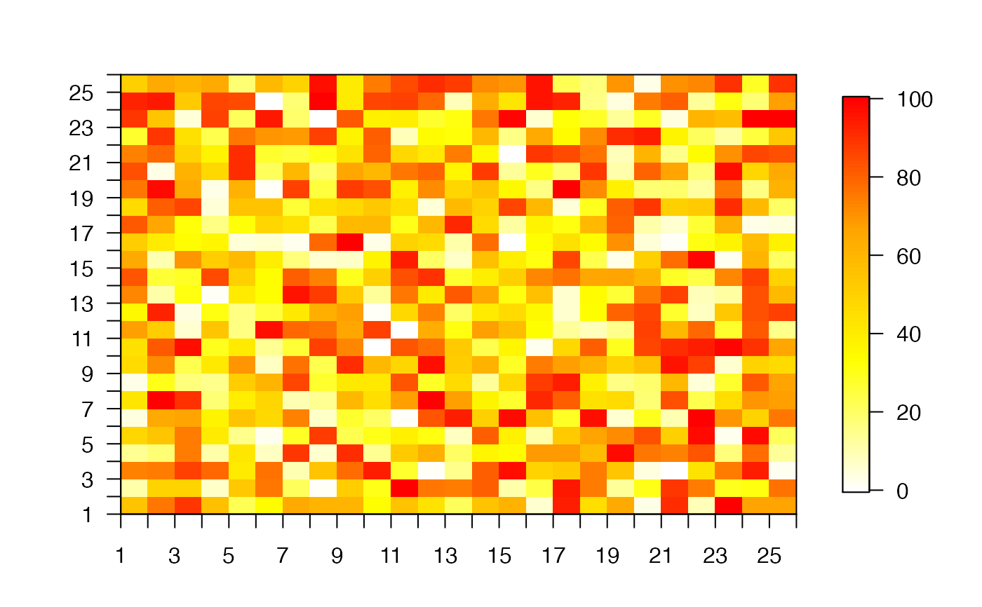
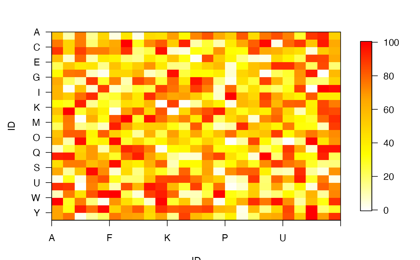
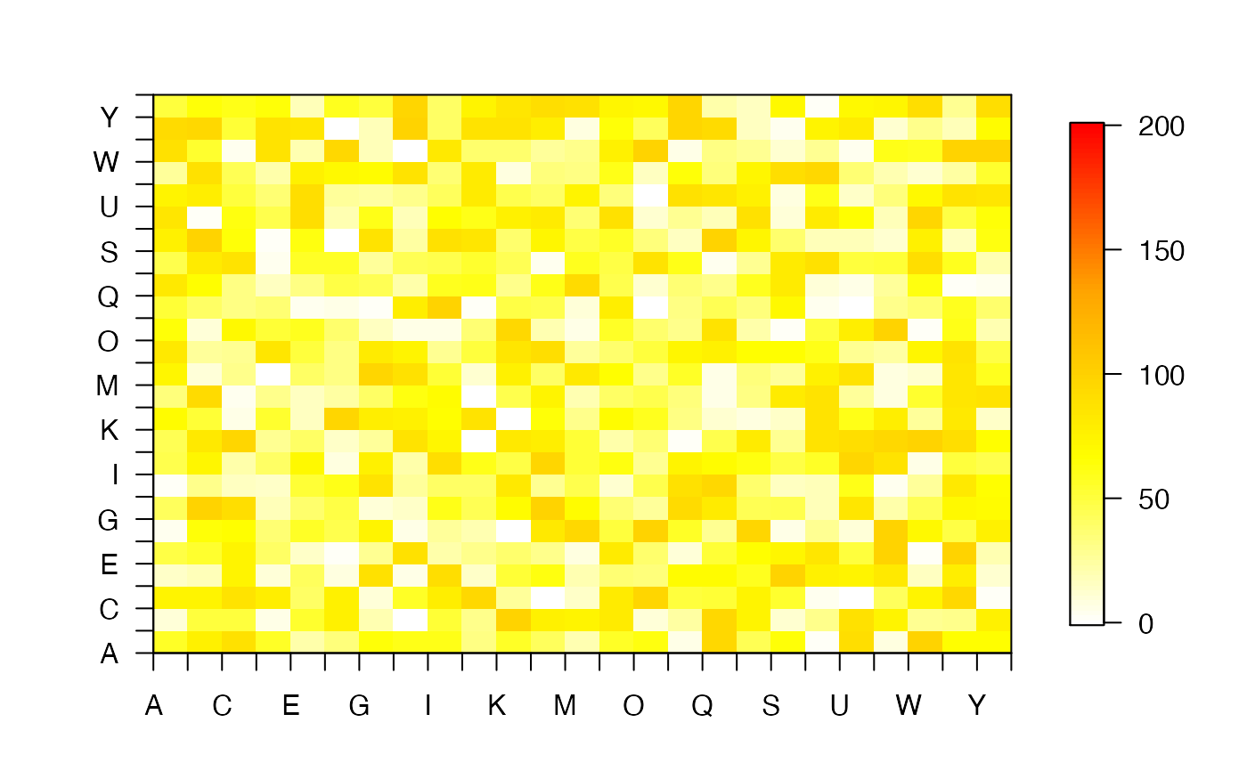
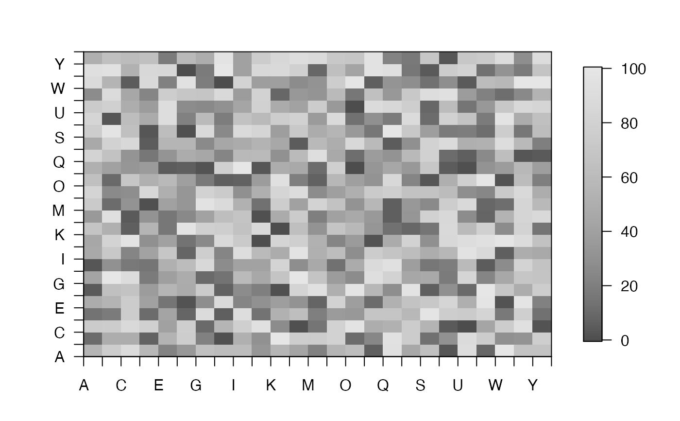
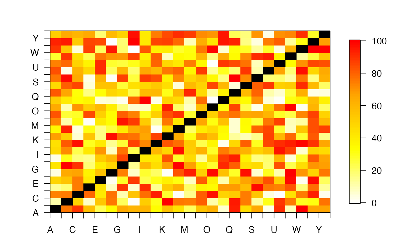
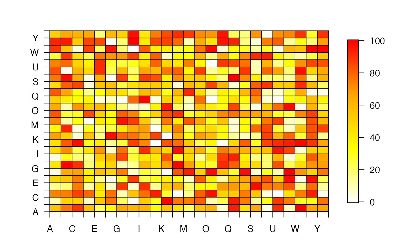
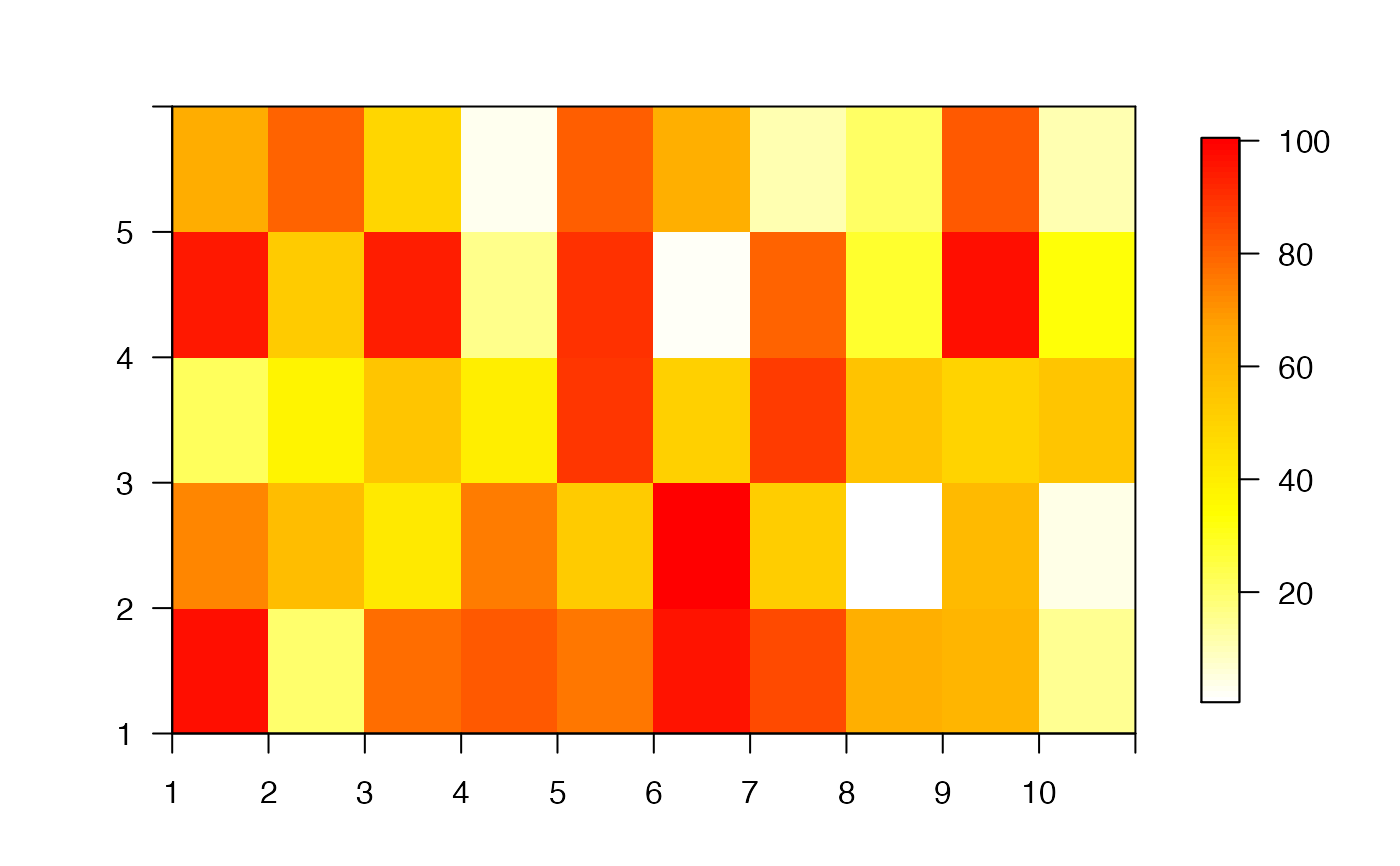
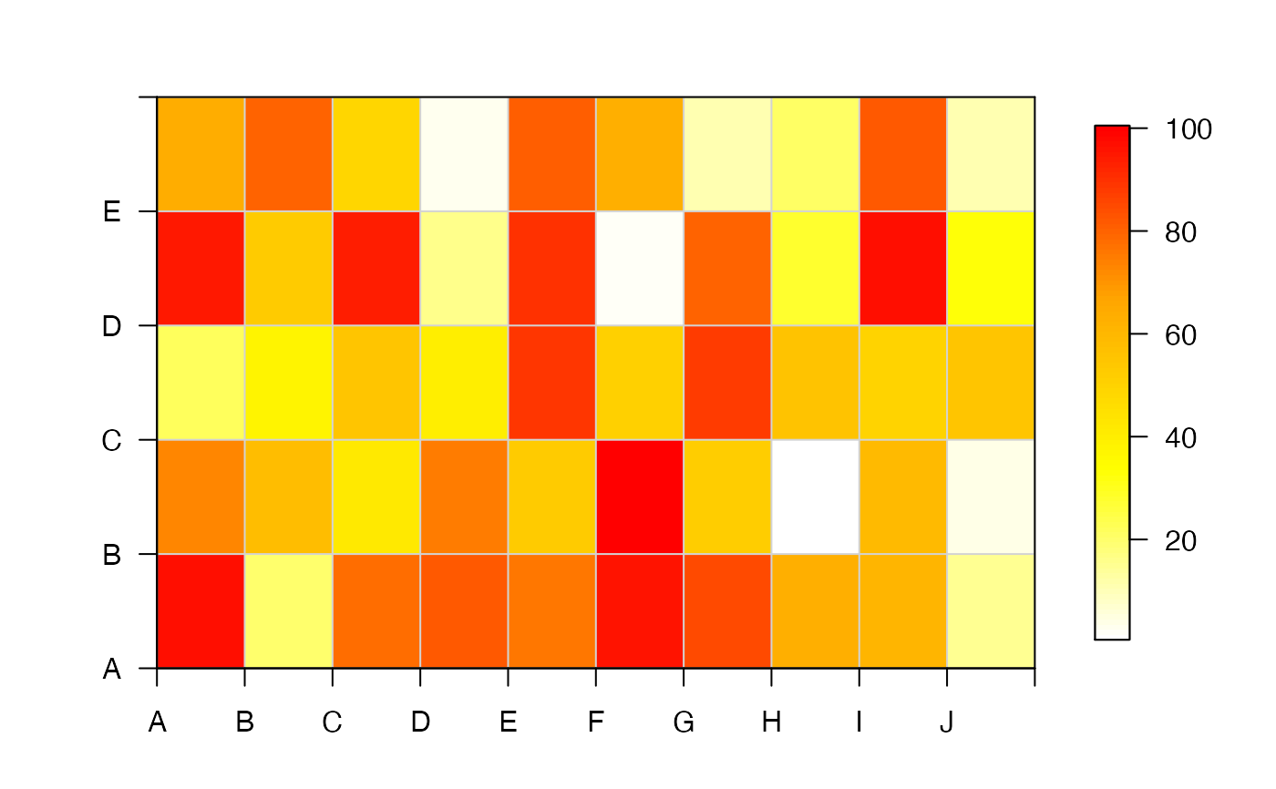
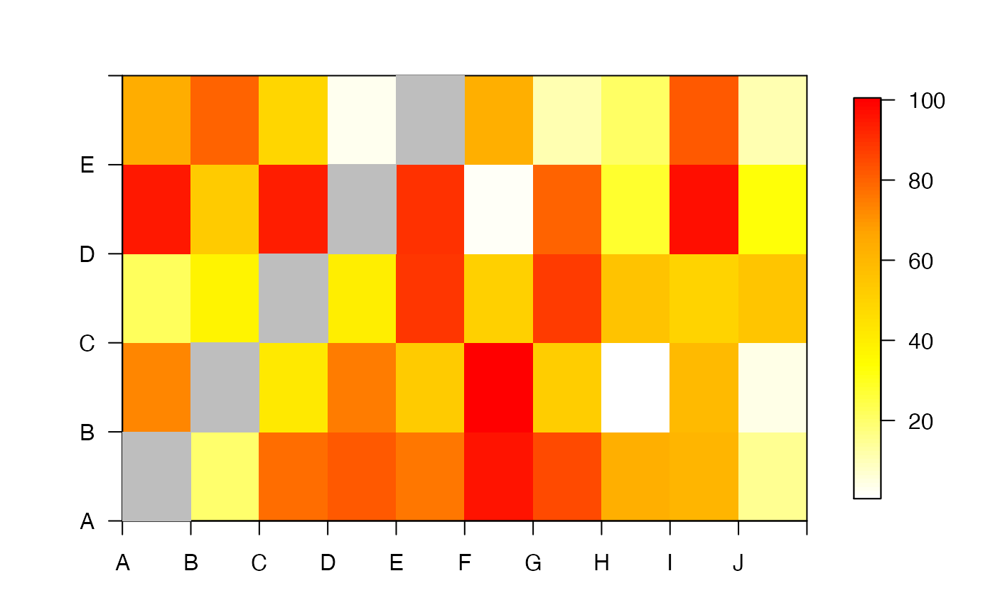
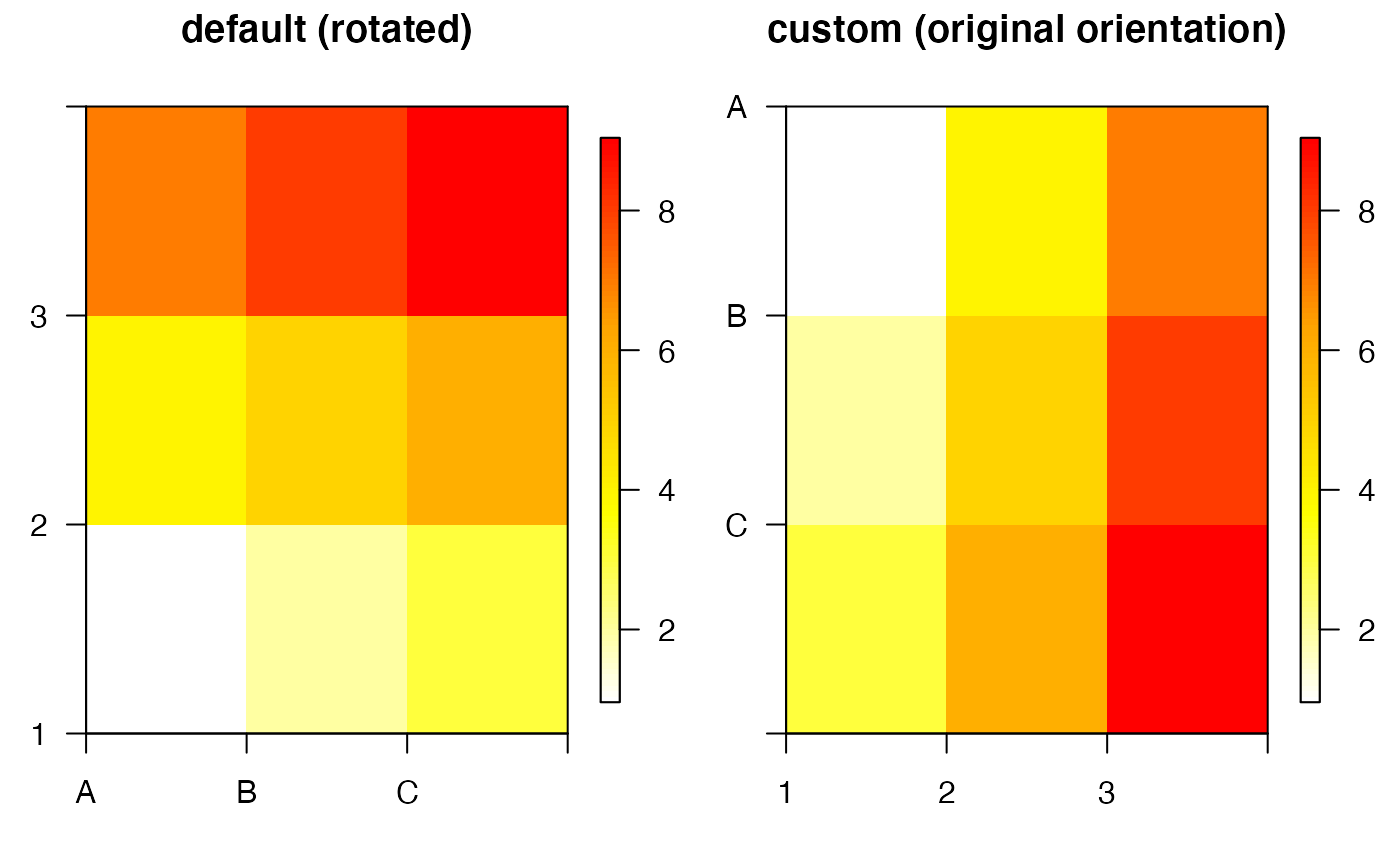
Examples

#### Define an example square matrix
n <- 25
mat <- matrix(sample(0:100, size = n^2, replace = TRUE), ncol = 25, nrow = 25)

#### Example (1): The default options
pretty_mat(mat)

#### Example (2): Customisation
# Adjust labelling and note how under the default settings the plot
# ... is rotated by 90 degrees counter-clockwise
rownames(mat) <- colnames(mat) <- LETTERS[1:nrow(mat)]
pretty_mat(mat)
pretty_mat(mat, xlab = "ID", ylab = "ID")
# Adjust the number of labels
pretty_mat(mat, xlab = "ID", ylab = "ID",
           xtick_every_n = 5, ytick_every_n = 2)
# Compare to plot with retained orientation
pretty_mat(mat, xlab = "ID", ylab = "ID",
           xtick_every_n = 5, ytick_every_n = 2,
           retain_orientation = TRUE)
# Adjust z limits
pretty_mat(mat, zlim = c(0, 200))
# Adjust colour scheme
pretty_mat(mat, col = grey.colors(100))
# Colour the diagonal (useful for symmetric square matrices)
pretty_mat(mat, col_diag = "black")
# Add a grid using default options
pretty_mat(mat, grid = list())
# Customise the grid
pretty_mat(mat, grid = list(col = "black", lty = 1))

#### Example (3) Rectangular matrices function similarly
# Define matrix
n1 <- 5; n2 <- 10
mat <- matrix(sample(0:100, size = n1*n2, replace = TRUE), ncol = n1, nrow = n2)
utils::str(mat)
#>  int [1:10, 1:5] 97 20 78 82 76 96 85 63 61 15 ...
# Visualise matrix with default options
pretty_mat(mat)
# Adjust names
rownames(mat) <- LETTERS[1:nrow(mat)]
colnames(mat) <- LETTERS[1:ncol(mat)]
pretty_mat(mat)
# Other options can be implemented as above
pretty_mat(mat, grid = list(lty = 1))
# However, adding colours along the diagonal may not make sense for asymmetric matrices
pretty_mat(mat, col_diag = "grey")

#' #### Example (4): Understanding the retain_orientation argument:
# ... Under the default option (retain_orientation is FALSE), R plots a
# ... 90 degree counter-clockwise rotation of the conventional
# ... printed layout of a matrix. This can be difficult to interpret.
# ... retain_orientation = TRUE ensures the matrix is plotted in the
# ... correct orientation
# Define a simple matrix
n <- 3
mat <- matrix(1:9, ncol = 3, nrow = 3)
# Distinguish row names from column names
rownames(mat) <- LETTERS[1:ncol(mat)]
# Check matrix
mat
#>   [,1] [,2] [,3]
#> A    1    4    7
#> B    2    5    8
#> C    3    6    9
# Visualise 'default' versus 'expected' matrix
pp <- par(mfrow = c(1, 2))
pretty_mat(mat, retain_orientation = FALSE, main = "default (rotated)")
pretty_mat(mat, retain_orientation = TRUE, main = "custom (original orientation)")
par(pp)