Observation model plots

plot() methods for observation models (see ModelObs).

Usage

# S3 method for class 'ModelObsAcousticLogisTrunc'
plot(x, .sensor_id, .par = list(), ...)

# S3 method for class 'ModelObsDepthUniformSeabed'
plot(x, .seabed = 100, .par = list(), ...)

# S3 method for class 'ModelObsDepthNormalTruncSeabed'
plot(x, .seabed = 100, .par = list(), ...)

# S3 method for class 'ModelObsContainer'
plot(x, .radius, .par = list(), ...)

Arguments

x

A named list of observation model parameters, including a ModelObs S3 label (from a model_obs_*() function).

.sensor_id, .radius, .seabed

Model-specific parameters:

• .sensor_id: For plot.ModelObsAcousticLogisTrunc(), .sensor_id controls the sensors (receivers) for which detection probability curves are shown:

  • missing (default) plots all unique curves;

  • An integer vector of sensor IDs plots curves for selected sensors;

  • NULL plots curves for all sensors;

• .radius: For plot.ModelObsContainer(), .radius controls the radii for which distributions are shown:

  • missing (default) plots distributions for first three unique radii;

  • A vector of radii plots curves for selected radii;

  • NULL plots distributions for all radii;

• .seabed: For plot.ModelObsDepth*Seabed(), .seabed is the seabed depth at which distributions are plotted.

.par

Graphical parameters:

• NULL uses current graphical parameters;

• list() uses default graphical parameters;

• A named list of arguments, passed to par(), customises parameters;

...

Additional arguments, passed to plot().

Value

The functions produce a plot. invisible(NULL) is returned.

Details

Observation model (ModelObs) structures are objects that define the parameters of an observation model. The model specifies the probability of an observation (e.g., a particular depth record) given the data (e.g., a depth measurement).

• plot.ModelObsAcousticLogisTrunc() plots detection probability as a function of distance from a receiver;

• plot.ModelObsDepthUniformSeabed() plots a uniform distribution for the probability of a depth observation around a particular .seabed depth;

• plot.ModelObsDepthNormalTruncSeabed() plot a truncated normal distribution for the probability of a depth observation around a particularly .seabed depth;

• plot.ModelObsContainer() plots a uniform distribution for the probability of a future observation (e.g., detection) given the maximum possible distance (container radius) from the container centroid (e.g., receiver), and a maximum movement speed, at the current time;

Author

Edward Lavender

Examples

if (patter_run(.julia = TRUE, .geospatial = FALSE)) {

  library(data.table)

  julia_connect()

  #### Example (1): ModelObsAcousticLogisTrunc
  # Plot unique detection-probability function(s)
  dat_moorings |>
    model_obs_acoustic_logis_trunc() |>
    plot()
  # Plot functions for selected sensors
  dat_moorings |>
    model_obs_acoustic_logis_trunc() |>
    plot(.sensor_id = unique(dat_moorings$receiver_id)[1:10])

  #### Example (2): ModelObsDepthUniformSeabed
  data.table(sensor_id = 1L, depth_shallow_eps = 10, depth_deep_eps = 10) |>
    model_obs_depth_uniform_seabed() |>
    plot()
  data.table(sensor_id = 1L, depth_shallow_eps = 10, depth_deep_eps = 10) |>
    model_obs_depth_uniform_seabed() |>
    plot(.seabed = 50)

  #### Example (3): ModelObsDepthSeabedNormalTrunc
  data.table(sensor_id = 1L, depth_sigma = 10, depth_deep_eps = 10) |>
    model_obs_depth_normal_trunc_seabed() |>
    plot()
  data.table(sensor_id = 1L, depth_sigma = 100, depth_deep_eps = 50) |>
    model_obs_depth_normal_trunc_seabed() |>
    plot(.seabed = 150)

  #### Example (4): ModelObsContainer
  # Define detections (1)
  detections <- dat_detections[individual_id == individual_id[1], ]
  # Assemble acoustic observations (0, 1) for a given timeline
  timeline   <- assemble_timeline(list(detections), .step = "2 mins")[1:100]
  acoustics  <- assemble_acoustics(.timeline   = timeline,
                                   .detections = detections,
                                   .moorings   = dat_moorings)
  # Assemble acoustic containers
  containers <- assemble_acoustics_containers(.timeline = timeline,
                                              .acoustics = acoustics,
                                              .mobility = 750)
  # Plot a few example distributions
  containers$forward |>
    model_obs_container() |>
    plot()

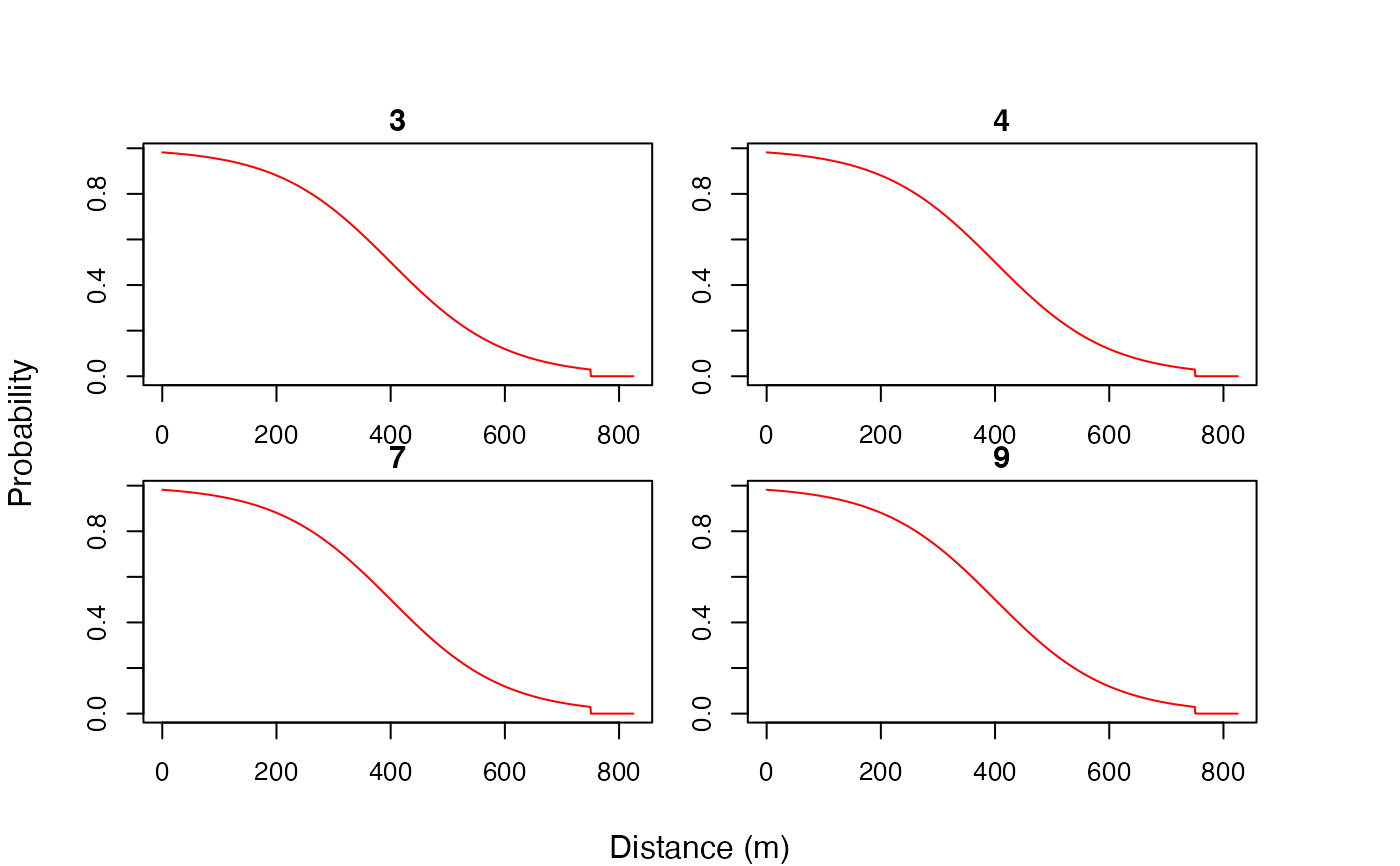
  #### Example (5): Customise plot layout via `.par`
  dat_moorings |>
    model_obs_acoustic_logis_trunc() |>
    plot(.sensor_id = unique(dat_moorings$receiver_id)[1:4],
         .par = list(mfrow = c(2, 2)))

  #### Example (6): Customise plot properties via `...`
  dat_moorings |>
    model_obs_acoustic_logis_trunc() |>
    plot(.sensor_id = unique(dat_moorings$receiver_id)[1:4],
         .par = list(mfrow = c(2, 2),
                     oma = c(3, 3, 3, 3),
                     mar = c(1.5, 1.5, 1.5, 1.5)),
         xlab = "", ylab = "", col = "red")
  mtext(side = 1, "Distance (m)", line = -1, outer = TRUE)
  mtext(side = 2, "Probability", line = -1, outer = TRUE)

}
#> `patter::julia_connect()` called @ 2025-04-22 09:31:49... 
#> ... Running `Julia` setup via `JuliaCall::julia_setup()`... 
#> ... Validating Julia installation... 
#> ... Setting up Julia project... 
#> ... Handling dependencies... 
#> ... `Julia` set up with 11 thread(s). 
#> `patter::julia_connect()` call ended @ 2025-04-22 09:31:49 (duration: ~0 sec(s)).