Add a regression line and an error envelope to a plot

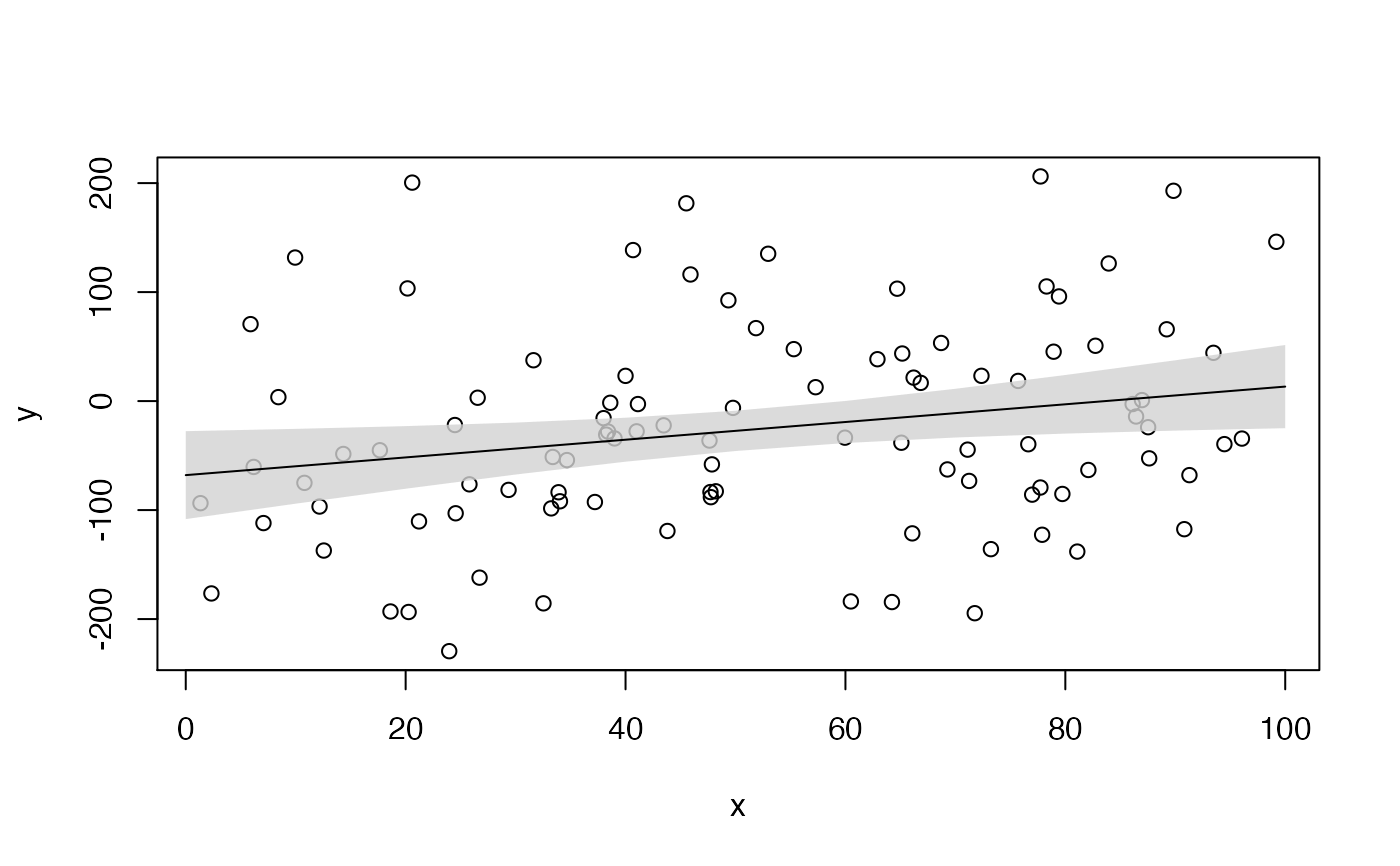
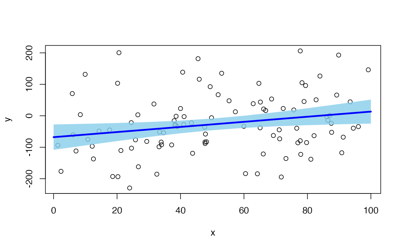
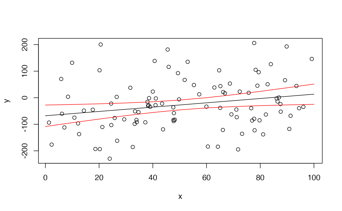
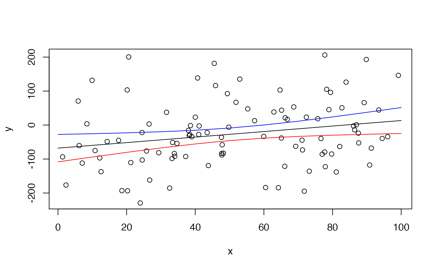
This function adds regression lines and associated error envelopes (e.g., confidence intervals, CIs) to plots. This function is designed to streamline plotting codes. Confidence intervals can be added as a polygon or as lines (with or without the fitted line added ontop). For large datasets, adding confidence intervals with lines is much faster.

add_error_envelope(
  x,
  ci = list(),
  type = "poly",
  add_ci = list(col = scales::alpha("lightgrey", 0.8), border = FALSE),
  add_fit = list(col = "black", lwd = 1, lty = 1),
  ...
)

Arguments

x	A numeric vector defining the x values at which fitted values/CIs will be plotted.
ci	A named list with fitted values (optional) and lower and upper CIs (i.e. ci$fit, ci$lowerCI, ci$upperCI). This can be created by list_CIs.
type	A character defining the method by which CIs will be added to a plot: as lines (type = "l" or type = "lines") or as a shaded polygon ("poly"). For large datasets, type = "lines" is much faster.
add_ci	(optional) A named list of arguments to customise the appearance of the confidence envelope, passed to lines or polygon depending on type. add_ci = NULL suppresses this option; add_ci = list() implements default arguments. If type = "lines", then two nested lists can be included to specify the lower and upper CI lines differently, if desired.
add_fit	(optional) A named list of arguments to customise the appearence of the fitted line. add_fit = NULL suppresses this option; add_fit = list() implements default arguments.
...	Additional arguments: none are currently implemented but depreciated arguments (CI, fCI, CI_gp and fitted_gp) are accepted (with a warning) via ....

Value

The function adds model predictions to a plot.

Details

The function is designed for continuous explanatory variables. add_error_bars is used for discrete explanatory variables to add fitted values and associated errors to plots.

Author

Edward Lavender

Examples

# Define some data for a model
set.seed(1)
x <- runif(100, 0, 100)
y <- rnorm(100, 0.5*x - 50, 100)
# Define model
m1 <- lm(y ~ x)
# Define predictions
xp <-  seq(0, 100, by = 10)
p <- predict(m1, newdata = data.frame(x = xp), se.fit = TRUE)
# List CIs
CIs <- list_CIs(pred = p, plot_suggestions = FALSE)
# Visualise
plot(x, y)

#### Example (1):
# Add predicted CIs as a polygon and add fitted line ontop using default graphical parameters
# Note that type = "poly", and add_fitted = TRUE do not need to be supplied
# ... since these are the default options
add_error_envelope(x = xp, ci = CIs)

#### Example (2):
# Add predicted CIs as a polygon and add fitted lines with user-specified parameters
plot(x, y)
add_error_envelope(x = xp,
                   ci = CIs,
                   add_ci = list(col = scales::alpha("skyblue", 0.8), border = FALSE),
                   add_fit = list(col = "blue", lwd = 3, lty = 1)
                   )

#### Example (3):
# Add predicted CIs as lines, where both upper and lower CIs have identical graphical parameters
plot(x, y)
add_error_envelope(x = xp,
                   ci = CIs,
                   type = "lines",
                   add_ci = list(col = "red")
                   )

#### Example (4):
# Control lower and upper CI lines independently in a nested list
# The first element is the lower CI; the second element is the upper CI
plot(x, y)
add_error_envelope(x = xp,
                   ci = CIs,
                   type = "lines",
                   add_ci = list(list(col = "red"), list(col = "blue"))
                   )