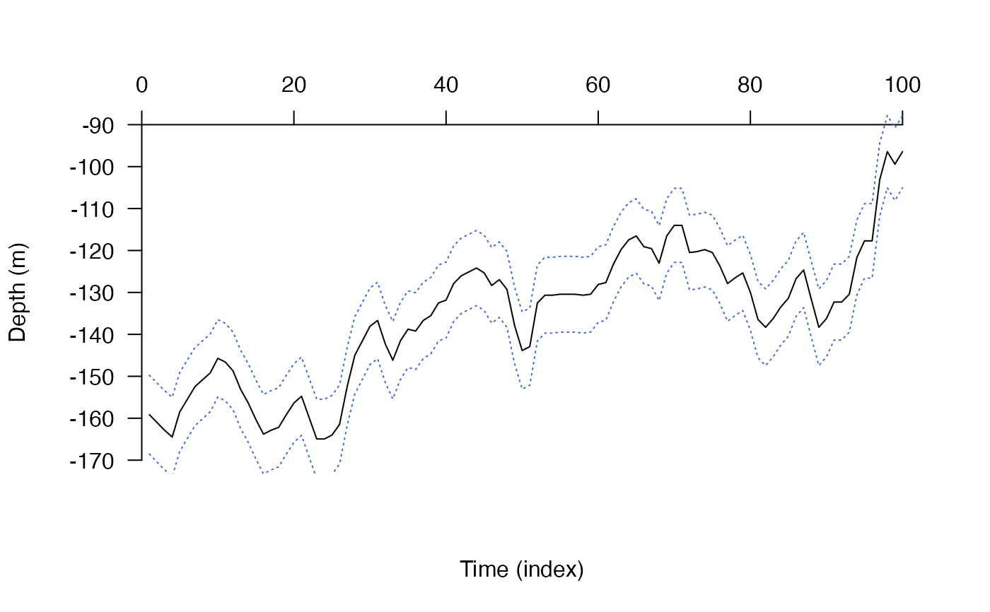
This function implements the depth-contour (DC) algorithm. This algorithm relates one-dimensional depth time series to a two-dimensional bathymetry surface to determine the extent to which different parts of an area might have (or have not) been used, or effectively represent occupied depths, over time. Given a sequence of depth observations (archival) from a tagged animal and a measurement error parameter (calc_depth_error), at each time step the function determines the cells on a bathymetry raster (bathy) that match the observed depth*. Across all time steps, matches are summed to produce a single map representing the number of occasions when the depth in each cell matched the observed depth.
Arguments
- archival
A dataframe of depth time series (for a single individual). At a minimum, this should contain a column named `depth' with depth observations. Depth should be recorded using absolute values in the same units as the bathymetry (
bathy, see below).- bathy
A
rasterof the bathymetry in an area within which the animal is likely to have been located over the study. Bathymetry values should be recorded as absolute values and in the same units as for depths (seearchival).- plot_ts
A logical input that defines whether or not to the depth time series before the algorithm is initiated.
- calc_depth_error
A function that returns the depth errors around a vector of depths. The function should accept vector of depths (from
archival$depth) and return a matrix, with one row for each (lower and upper) error and one one column for each depth (if the error varies with depth). For each depth, the two numbers are added to the observed depth to define the range of depths on the bathymetry raster (bathy) that the individual could plausibly have occupied at any time. Since the depth errors are added to the individual's depth, the first number should be negative (i.e., the individual could have been shallower that observed) and the second positive (i.e., the individual could have been deeper than observed). The appropriate form forcalc_depth_errordepends on the species (pelagic versus demersal/benthic species), the measurement error for the depth observations inarchivaland bathymetry (bathy) data, as well as the tidal range (m) across the area (over the duration of observations). For example, for a pelagic species, the constant functioncalc_depth_error = function(...) matrix(c(-2.5, Inf)implies that the individual could have occupied bathymetric cells that are deeper than the observed depth + (-2.5) m and shallower than Inf m (i.e. the individual could have been in any location in which the depth was deeper than the shallow depth limit for the individual). In contrast, for a benthic species, the constant functioncalc_depth_error = function(...) matrix(c(-2.5, 2.5), nrow = 2)implies that the individual could have occupied bathymetric cells whose depth lies within the interval defined by the observed depth + (-2.5) and + (+2.5) m.- check_availability
A logical input that defines whether or not to record explicitly, for each time step, whether or not there were any cells on
bathythat matched the observed depth (within the bounds defined bycalc_depth_error).- normalise
A logical variable that defines whether or not to normalise the map of possible locations at each time step so that their scores sum to one.
- save_record_spatial
An integer vector that defines the time steps for which to return time step-specific and cumulative maps of the individual's possible locations.
save_record_spatial = 0suppresses the return of this information andsave_record_spatial = NULLreturns this information for all time steps.- write_record_spatial_for_pf
(optional) A named list, passed to
writeRaster, to save therasterof the individual's possible positions at each time step to file. The `filename' argument should be the directory in which to save files. Files are named by archival time steps as `arc_1', `arc_2' and so on.- save_args
A logical input that defines whether or not to save the list of function inputs in the returned object.
- verbose
A logical variable that defines whether or not to print messages to the console or to file to relay function progress. If
con = "", messages are printed to the console; otherwise, they are written to file (see below).- con
If
verbose = TRUE,conis character string that defines how messages relaying function progress are returned. Ifcon = "", messages are printed to the console (unless redirected bysink). Otherwise,condefines the full pathway to a .txt file (which can be created on-the-fly) into which messages are written to relay function progress.- split, cl, varlist
(optional) Parallelisation options.
splitis an integer which, if supplied, splits thearchivaldataframe everynth row into chunks†. The algorithm is applied sequentially within each chunk (if applicable) and chunk-wise maps can be summed afterwards to create a single map of space use. The advantage of this approach is that chunks can be analysed in parallel, viaclandvarlist, while memory use is minimised.clis (a) a cluster object frommakeClusteror (b) an integer that defines the number of child processes.varlistis a character vector of variables for export (seecl_export). Exported variables must be located in the global environment. If a cluster is supplied, the connection to the cluster is closed within the function (seecl_stop). For further information, seecl_lapplyandflapper-tips-parallel.
Value
The function returns an acdc_archive-class object. If a connection to write files has also been specified, messages are also written to file relaying function progress.
Details
This algorithm can be applied to both pelagic species (which must be in an area where the depth is at least as deep as the observed depth) and benthic/demersal species (which must be in an area relatively close in depth to the observed depth). However, the results are likely to be much more precise for benthic species because depth observations for benthic animals are typically more informative about a tagged animal's possible location(s) than for pelagic species.
*Location probability could be weighted by the proximity between the observed depth and the depths of cells within the range defined by the observed depth and the measurement error (i.e., archival$depth[1] + calc_depth_error(archival$depth[1])[1], archival$depth[1] + calc_depth_error(archival$depth[1])[2]), but this is not currently implemented.
†Under the default options (split = NULL), the function starts with a blank map of the area and iterates over each time step, adding the `possible positions' of the individual to the map at each step. By continuously updating a single map, this approach is slow but minimises memory requirements. An alternative approach is to split the time series into chunks, implement an iterative approach within each chunk, and then join the maps for each chunk. This is implemented by split (plus acdc_simplify).
See also
acdc_simplify simplifies the outputs of the algorithm. acdc_plot_trace, acdc_plot_record and acdc_animate_record provide plotting routines. dcq implements a faster version of this algorithm termed the `quick depth-contour' (DCQ) algorithm. Rather than considering the depth interval that the individual could have occupied at each time step, the DCQ algorithm considers a sequence of depth bins (e.g., 10 m bins), isolates these on the bathymetry raster (bathy) and counts the number of matches in each cell. The DCPF algorithm (see pf) extends the DC algorithm via particle filtering to reconstruct possible movement paths over bathy. The ACDC algorithm (see acdc) extends the depth-contour algorithm by integrating information from acoustic detections of individuals at each time step to restrict the locations in which depth contours are identified.
Examples
#### Define depth time series for examples
# We will use a sample depth time series for one individual
# We will select a small sample of observations for example speed
depth <- dat_archival[dat_archival$individual_id == 25, ][1:100, ]
#### Example (1): Implement algorithm with default options
## Implement algorithm
out_dc <- dc(archival = depth, bathy = dat_gebco)
#> flapper::dc() called (@ 2023-08-29 15:37:35)...
#> ... Setting up function...
#> 'calc_depth_error' function taken to be independent of depth.
#> ... Implementing calc_depth_error()...
#> ... Plotting movement time series (for each chunk)...
 #> ... Implementing algorithm over time steps...
#> ... flapper::dc() call completed (@ 2023-08-29 15:37:40) after ~0.09 minutes.
## dc() returns a named list that is an 'acdc_archive' class object
summary(out_dc)
#> Length Class Mode
#> archive 1 -none- list
#> ts_by_chunk 1 -none- list
#> time 4 data.frame list
#> args 14 -none- list
# ... archive elements contain the key information from the algorithm
# ... ts_by_chunk contains the time series for each chunk
# ... time contains a dataframe of the algorithm's progression
# ... args contains a list of user inputs
## Simplify outputs via acdc_simplify()
dc_summary <- acdc_simplify(out_dc, type = "dc")
#> acdc_simplify() implemented for type = 'dc'.
summary(dc_summary)
#> Length Class Mode
#> map 4218 RasterLayer S4
#> record 100 -none- list
#> time 4 data.frame list
#> args 14 -none- list
#> chunks 0 -none- NULL
#> simplify 1 -none- logical
## Examine time-specific maps via acdc_plot_record()
acdc_plot_record(dc_summary)
#> flapper::acdc_plot_record() called...
#> ... Checking function inputs...
#> ... Defining data for background plot...
#> `add_containers = NULL` implemented: 'record' does not contain containers (`container_c` element).
#> ... Setting plotting window...
#> ... Making plots for each time step ...
#> Warning: Nothing to summarize if you provide a single RasterLayer; see cellStats
#> ... Implementing algorithm over time steps...
#> ... flapper::dc() call completed (@ 2023-08-29 15:37:40) after ~0.09 minutes.
## dc() returns a named list that is an 'acdc_archive' class object
summary(out_dc)
#> Length Class Mode
#> archive 1 -none- list
#> ts_by_chunk 1 -none- list
#> time 4 data.frame list
#> args 14 -none- list
# ... archive elements contain the key information from the algorithm
# ... ts_by_chunk contains the time series for each chunk
# ... time contains a dataframe of the algorithm's progression
# ... args contains a list of user inputs
## Simplify outputs via acdc_simplify()
dc_summary <- acdc_simplify(out_dc, type = "dc")
#> acdc_simplify() implemented for type = 'dc'.
summary(dc_summary)
#> Length Class Mode
#> map 4218 RasterLayer S4
#> record 100 -none- list
#> time 4 data.frame list
#> args 14 -none- list
#> chunks 0 -none- NULL
#> simplify 1 -none- logical
## Examine time-specific maps via acdc_plot_record()
acdc_plot_record(dc_summary)
#> flapper::acdc_plot_record() called...
#> ... Checking function inputs...
#> ... Defining data for background plot...
#> `add_containers = NULL` implemented: 'record' does not contain containers (`container_c` element).
#> ... Setting plotting window...
#> ... Making plots for each time step ...
#> Warning: Nothing to summarize if you provide a single RasterLayer; see cellStats
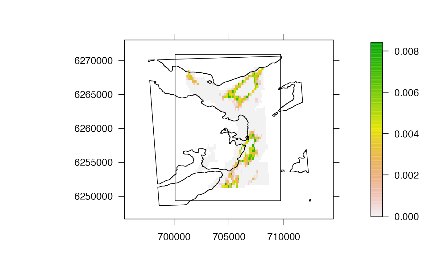
 ## Examine overall map via a raster* plotting function
# Each cell shows expected proportion of time steps spent in each cell
prettyGraphics::pretty_map(
add_rasters = list(x = dc_summary$map),
add_polys = list(x = dat_coast)
)
#> prettyGraphics::pretty_map() CRS taken as: '+proj=utm +zone=29 +datum=WGS84 +units=m +no_defs'.
## Examine overall map via a raster* plotting function
# Each cell shows expected proportion of time steps spent in each cell
prettyGraphics::pretty_map(
add_rasters = list(x = dc_summary$map),
add_polys = list(x = dat_coast)
)
#> prettyGraphics::pretty_map() CRS taken as: '+proj=utm +zone=29 +datum=WGS84 +units=m +no_defs'.
 # Convert counts on map to percentages
prettyGraphics::pretty_map(
add_rasters =
list(
x = dc_summary$map / nrow(depth) * 100,
zlim = c(0, 100)
),
add_polys = list(x = dat_coast)
)
#> prettyGraphics::pretty_map() CRS taken as: '+proj=utm +zone=29 +datum=WGS84 +units=m +no_defs'.
# Convert counts on map to percentages
prettyGraphics::pretty_map(
add_rasters =
list(
x = dc_summary$map / nrow(depth) * 100,
zlim = c(0, 100)
),
add_polys = list(x = dat_coast)
)
#> prettyGraphics::pretty_map() CRS taken as: '+proj=utm +zone=29 +datum=WGS84 +units=m +no_defs'.
 # Check for occasions when the individual's depth was not consistent
# ... with the depth data for the area and the depth error e.g., possibly
# ... due to movement beyond this area:
any(do.call(rbind, lapply(dc_summary$record, function(elm) elm$dat))$availability == FALSE)
#> [1] FALSE
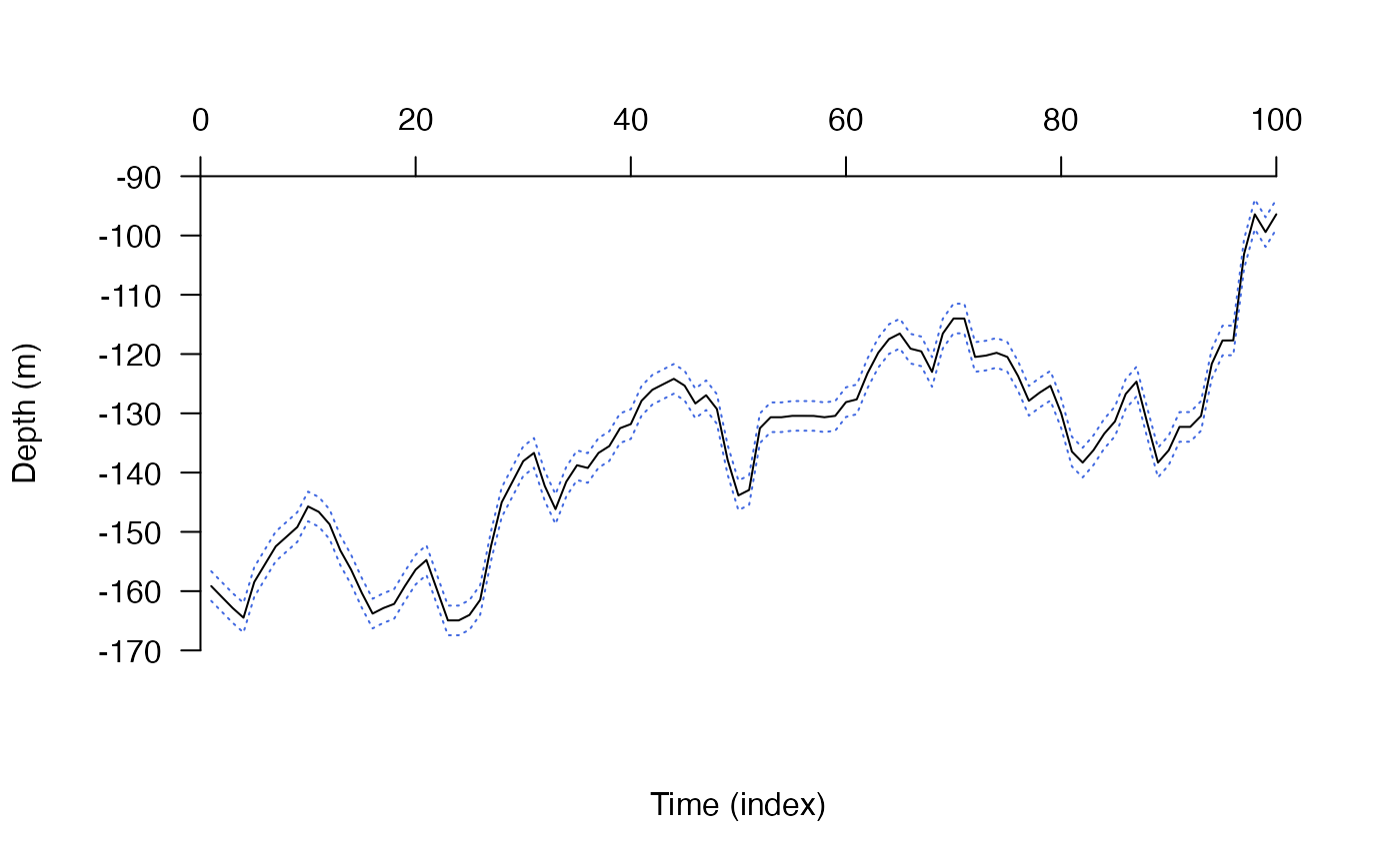
#### Example (2): Implement depth error functions that depend on depth
## Here, we will define a calc_depth_error function that depends on:
# ... tag error
# ... tidal range
# ... a depth-dependent bathymetry error
cde <- function(depth) {
e <- 4.77 + 2.5 + sqrt(0.5^2 + (0.013 * depth)^2)
e <- matrix(c(-e, e), nrow = 2)
return(e)
}
# Vectorise function over depths (essential)
cde <- Vectorize(cde)
## Implement algorithm with depth-dependent error
out_dc <- dc(archival = depth, bathy = dat_gebco, calc_depth_error = cde)
#> flapper::dc() called (@ 2023-08-29 15:37:41)...
#> ... Setting up function...
#> 'calc_depth_error' taken to depend on depth.
#> ... Implementing calc_depth_error()...
#> ... Plotting movement time series (for each chunk)...
# Check for occasions when the individual's depth was not consistent
# ... with the depth data for the area and the depth error e.g., possibly
# ... due to movement beyond this area:
any(do.call(rbind, lapply(dc_summary$record, function(elm) elm$dat))$availability == FALSE)
#> [1] FALSE
#### Example (2): Implement depth error functions that depend on depth
## Here, we will define a calc_depth_error function that depends on:
# ... tag error
# ... tidal range
# ... a depth-dependent bathymetry error
cde <- function(depth) {
e <- 4.77 + 2.5 + sqrt(0.5^2 + (0.013 * depth)^2)
e <- matrix(c(-e, e), nrow = 2)
return(e)
}
# Vectorise function over depths (essential)
cde <- Vectorize(cde)
## Implement algorithm with depth-dependent error
out_dc <- dc(archival = depth, bathy = dat_gebco, calc_depth_error = cde)
#> flapper::dc() called (@ 2023-08-29 15:37:41)...
#> ... Setting up function...
#> 'calc_depth_error' taken to depend on depth.
#> ... Implementing calc_depth_error()...
#> ... Plotting movement time series (for each chunk)...
 #> ... Implementing algorithm over time steps...
#> ... flapper::dc() call completed (@ 2023-08-29 15:37:45) after ~0.08 minutes.
#### Example (3): Write timestep-specific maps of allowed positions to file
out_dc <- dc(
archival = depth, bathy = dat_gebco,
write_record_spatial_for_pf = list(filename = tempdir())
)
#> flapper::dc() called (@ 2023-08-29 15:37:45)...
#> ... Setting up function...
#> 'calc_depth_error' function taken to be independent of depth.
#> '/' added to the directory inputted to the argument 'write_record_spatial_for_pf$filename' ('/var/folders/nl/ygb3g6tj24z06jddbqqhj6hw0000gn/T//Rtmpwb5KFV').
#> ... Implementing calc_depth_error()...
#> ... Plotting movement time series (for each chunk)...
#> ... Implementing algorithm over time steps...
#> ... flapper::dc() call completed (@ 2023-08-29 15:37:45) after ~0.08 minutes.
#### Example (3): Write timestep-specific maps of allowed positions to file
out_dc <- dc(
archival = depth, bathy = dat_gebco,
write_record_spatial_for_pf = list(filename = tempdir())
)
#> flapper::dc() called (@ 2023-08-29 15:37:45)...
#> ... Setting up function...
#> 'calc_depth_error' function taken to be independent of depth.
#> '/' added to the directory inputted to the argument 'write_record_spatial_for_pf$filename' ('/var/folders/nl/ygb3g6tj24z06jddbqqhj6hw0000gn/T//Rtmpwb5KFV').
#> ... Implementing calc_depth_error()...
#> ... Plotting movement time series (for each chunk)...
 #> ... Implementing algorithm over time steps...
#> ... flapper::dc() call completed (@ 2023-08-29 15:37:53) after ~0.13 minutes.
list.files(tempdir())
#> [1] "1.png" "2.png"
#> [3] "25" "28"
#> [5] "35" "ACDC_algorithm_demo.html"
#> [7] "acdc_log.txt" "acdc_trace"
#> [9] "arc_1.grd" "arc_1.gri"
#> [11] "arc_10.grd" "arc_10.gri"
#> [13] "arc_100.grd" "arc_100.gri"
#> [15] "arc_11.grd" "arc_11.gri"
#> [17] "arc_12.grd" "arc_12.gri"
#> [19] "arc_13.grd" "arc_13.gri"
#> [21] "arc_14.grd" "arc_14.gri"
#> [23] "arc_15.grd" "arc_15.gri"
#> [25] "arc_16.grd" "arc_16.gri"
#> [27] "arc_17.grd" "arc_17.gri"
#> [29] "arc_18.grd" "arc_18.gri"
#> [31] "arc_19.grd" "arc_19.gri"
#> [33] "arc_2.grd" "arc_2.gri"
#> [35] "arc_20.grd" "arc_20.gri"
#> [37] "arc_21.grd" "arc_21.gri"
#> [39] "arc_22.grd" "arc_22.gri"
#> [41] "arc_23.grd" "arc_23.gri"
#> [43] "arc_24.grd" "arc_24.gri"
#> [45] "arc_25.grd" "arc_25.gri"
#> [47] "arc_26.grd" "arc_26.gri"
#> [49] "arc_27.grd" "arc_27.gri"
#> [51] "arc_28.grd" "arc_28.gri"
#> [53] "arc_29.grd" "arc_29.gri"
#> [55] "arc_3.grd" "arc_3.gri"
#> [57] "arc_30.grd" "arc_30.gri"
#> [59] "arc_31.grd" "arc_31.gri"
#> [61] "arc_32.grd" "arc_32.gri"
#> [63] "arc_33.grd" "arc_33.gri"
#> [65] "arc_34.grd" "arc_34.gri"
#> [67] "arc_35.grd" "arc_35.gri"
#> [69] "arc_36.grd" "arc_36.gri"
#> [71] "arc_37.grd" "arc_37.gri"
#> [73] "arc_38.grd" "arc_38.gri"
#> [75] "arc_39.grd" "arc_39.gri"
#> [77] "arc_4.grd" "arc_4.gri"
#> [79] "arc_40.grd" "arc_40.gri"
#> [81] "arc_41.grd" "arc_41.gri"
#> [83] "arc_42.grd" "arc_42.gri"
#> [85] "arc_43.grd" "arc_43.gri"
#> [87] "arc_44.grd" "arc_44.gri"
#> [89] "arc_45.grd" "arc_45.gri"
#> [91] "arc_46.grd" "arc_46.gri"
#> [93] "arc_47.grd" "arc_47.gri"
#> [95] "arc_48.grd" "arc_48.gri"
#> [97] "arc_49.grd" "arc_49.gri"
#> [99] "arc_5.grd" "arc_5.gri"
#> [101] "arc_50.grd" "arc_50.gri"
#> [103] "arc_51.grd" "arc_51.gri"
#> [105] "arc_52.grd" "arc_52.gri"
#> [107] "arc_53.grd" "arc_53.gri"
#> [109] "arc_54.grd" "arc_54.gri"
#> [111] "arc_55.grd" "arc_55.gri"
#> [113] "arc_56.grd" "arc_56.gri"
#> [115] "arc_57.grd" "arc_57.gri"
#> [117] "arc_58.grd" "arc_58.gri"
#> [119] "arc_59.grd" "arc_59.gri"
#> [121] "arc_6.grd" "arc_6.gri"
#> [123] "arc_60.grd" "arc_60.gri"
#> [125] "arc_61.grd" "arc_61.gri"
#> [127] "arc_62.grd" "arc_62.gri"
#> [129] "arc_63.grd" "arc_63.gri"
#> [131] "arc_64.grd" "arc_64.gri"
#> [133] "arc_65.grd" "arc_65.gri"
#> [135] "arc_66.grd" "arc_66.gri"
#> [137] "arc_67.grd" "arc_67.gri"
#> [139] "arc_68.grd" "arc_68.gri"
#> [141] "arc_69.grd" "arc_69.gri"
#> [143] "arc_7.grd" "arc_7.gri"
#> [145] "arc_70.grd" "arc_70.gri"
#> [147] "arc_71.grd" "arc_71.gri"
#> [149] "arc_72.grd" "arc_72.gri"
#> [151] "arc_73.grd" "arc_73.gri"
#> [153] "arc_74.grd" "arc_74.gri"
#> [155] "arc_75.grd" "arc_75.gri"
#> [157] "arc_76.grd" "arc_76.gri"
#> [159] "arc_77.grd" "arc_77.gri"
#> [161] "arc_78.grd" "arc_78.gri"
#> [163] "arc_79.grd" "arc_79.gri"
#> [165] "arc_8.grd" "arc_8.gri"
#> [167] "arc_80.grd" "arc_80.gri"
#> [169] "arc_81.grd" "arc_81.gri"
#> [171] "arc_82.grd" "arc_82.gri"
#> [173] "arc_83.grd" "arc_83.gri"
#> [175] "arc_84.grd" "arc_84.gri"
#> [177] "arc_85.grd" "arc_85.gri"
#> [179] "arc_86.grd" "arc_86.gri"
#> [181] "arc_87.grd" "arc_87.gri"
#> [183] "arc_88.grd" "arc_88.gri"
#> [185] "arc_89.grd" "arc_89.gri"
#> [187] "arc_9.grd" "arc_9.gri"
#> [189] "arc_90.grd" "arc_90.gri"
#> [191] "arc_91.grd" "arc_91.gri"
#> [193] "arc_92.grd" "arc_92.gri"
#> [195] "arc_93.grd" "arc_93.gri"
#> [197] "arc_94.grd" "arc_94.gri"
#> [199] "arc_95.grd" "arc_95.gri"
#> [201] "arc_96.grd" "arc_96.gri"
#> [203] "arc_97.grd" "arc_97.gri"
#> [205] "arc_98.grd" "arc_98.gri"
#> [207] "arc_99.grd" "arc_99.gri"
#> [209] "css" "dot_acdc_log_1.txt"
#> [211] "dot_acdc_log_2.txt" "dot_acdc_log_3.txt"
#> [213] "dot_acdc_log_4.txt" "dot_acdc_log_5.txt"
#> [215] "downlit" "file1217f158f0912"
#> [217] "file1217f1b0b625c" "file1217f2183169d"
#> [219] "file1217f619c87cc" "file1217f667087b8"
#> [221] "file1217f6772064" "file1217f67eddc54"
#> [223] "file1217f6b979424" "images"
#> [225] "js"
#### Example (4): Implement the algorithm in parallel
## Trial different options for 'split' and compare speed
# Approach (1)
at1 <- Sys.time()
cl <- parallel::makeCluster(2L)
parallel::clusterEvalQ(cl = cl, library(raster))
#> [[1]]
#> [1] "raster" "sp" "stats" "graphics" "grDevices" "utils"
#> [7] "datasets" "methods" "base"
#>
#> [[2]]
#> [1] "raster" "sp" "stats" "graphics" "grDevices" "utils"
#> [7] "datasets" "methods" "base"
#>
out_dc <- dc(
archival = depth,
bathy = dat_gebco,
plot_ts = FALSE,
split = 1,
cl = cl
)
#> flapper::dc() called (@ 2023-08-29 15:37:56)...
#> ... Setting up function...
#> 'calc_depth_error' function taken to be independent of depth.
#> ... Implementing calc_depth_error()...
#> ... Implementing algorithm over chunks...
#> ... flapper::dc() call completed (@ 2023-08-29 15:37:58) after ~0.04 minutes.
at2 <- Sys.time()
# Approach (2)
bt1 <- Sys.time()
cl <- parallel::makeCluster(2L)
parallel::clusterEvalQ(cl = cl, library(raster))
#> [[1]]
#> [1] "raster" "sp" "stats" "graphics" "grDevices" "utils"
#> [7] "datasets" "methods" "base"
#>
#> [[2]]
#> [1] "raster" "sp" "stats" "graphics" "grDevices" "utils"
#> [7] "datasets" "methods" "base"
#>
out_dc <- dc(
archival = depth,
bathy = dat_gebco,
plot_ts = FALSE,
split = 5,
cl = cl
)
#> flapper::dc() called (@ 2023-08-29 15:38:00)...
#> ... Setting up function...
#> 'calc_depth_error' function taken to be independent of depth.
#> ... Implementing calc_depth_error()...
#> ... Implementing algorithm over chunks...
#> ... flapper::dc() call completed (@ 2023-08-29 15:38:03) after ~0.04 minutes.
bt2 <- Sys.time()
# Compare timings
difftime(at2, at1)
#> Time difference of 5.250416 secs
difftime(bt2, bt1)
#> Time difference of 4.520967 secs
#### Example (5): Write messages to file via con
out_dc <- dc(
archival = depth, bathy = dat_gebco,
con = paste0(tempdir(), "/dc_log.txt")
)
#> /var/folders/nl/ygb3g6tj24z06jddbqqhj6hw0000gn/T//Rtmpwb5KFV/dc_log.txt does not exist: attempting to write file in specified directory...
#> ... Blank file successfully written to file.
#> 'calc_depth_error' function taken to be independent of depth.
readLines(paste0(tempdir(), "/dc_log.txt"))
#> [1] "flapper::dc() called (@ 2023-08-29 15:38:03)... "
#> [2] "... Setting up function... "
#> [3] "... Implementing calc_depth_error()... "
#> [4] "... Plotting movement time series (for each chunk)... "
#> [5] "... Implementing algorithm over time steps... "
#> [6] "... flapper::dc() call completed (@ 2023-08-29 15:38:07) after ~0.07 minutes. "
#### Example (6) Compare an automated vs. manual implementation of DC
## (A) Compare step-wise results for randomly select time steps
# Implement algorithm (using default calc_depth_error)
out_dc <- dc(
archival = depth,
bathy = dat_gebco,
save_record_spatial = NULL
)
#> flapper::dc() called (@ 2023-08-29 15:38:07)...
#> ... Setting up function...
#> 'calc_depth_error' function taken to be independent of depth.
#> ... Implementing calc_depth_error()...
#> ... Plotting movement time series (for each chunk)...
#> ... Implementing algorithm over time steps...
#> ... flapper::dc() call completed (@ 2023-08-29 15:38:12) after ~0.08 minutes.
# Compare results for randomly selected time steps to manual implementation
# ... with the same simple calc_depth_error model
pp <- graphics::par(mfrow = c(5, 2))
for (i in sample(1:nrow(depth), 5)) {
# Extract map created via dc()
raster::plot(out_dc$archive[[1]]$record[[i]]$spatial[[1]]$map_timestep)
# Compare to manual creation of map
raster::plot(dat_gebco >= depth$depth[i] - 2.5 & dat_gebco <= depth$depth[i] + 2.5)
}
#> ... Implementing algorithm over time steps...
#> ... flapper::dc() call completed (@ 2023-08-29 15:37:53) after ~0.13 minutes.
list.files(tempdir())
#> [1] "1.png" "2.png"
#> [3] "25" "28"
#> [5] "35" "ACDC_algorithm_demo.html"
#> [7] "acdc_log.txt" "acdc_trace"
#> [9] "arc_1.grd" "arc_1.gri"
#> [11] "arc_10.grd" "arc_10.gri"
#> [13] "arc_100.grd" "arc_100.gri"
#> [15] "arc_11.grd" "arc_11.gri"
#> [17] "arc_12.grd" "arc_12.gri"
#> [19] "arc_13.grd" "arc_13.gri"
#> [21] "arc_14.grd" "arc_14.gri"
#> [23] "arc_15.grd" "arc_15.gri"
#> [25] "arc_16.grd" "arc_16.gri"
#> [27] "arc_17.grd" "arc_17.gri"
#> [29] "arc_18.grd" "arc_18.gri"
#> [31] "arc_19.grd" "arc_19.gri"
#> [33] "arc_2.grd" "arc_2.gri"
#> [35] "arc_20.grd" "arc_20.gri"
#> [37] "arc_21.grd" "arc_21.gri"
#> [39] "arc_22.grd" "arc_22.gri"
#> [41] "arc_23.grd" "arc_23.gri"
#> [43] "arc_24.grd" "arc_24.gri"
#> [45] "arc_25.grd" "arc_25.gri"
#> [47] "arc_26.grd" "arc_26.gri"
#> [49] "arc_27.grd" "arc_27.gri"
#> [51] "arc_28.grd" "arc_28.gri"
#> [53] "arc_29.grd" "arc_29.gri"
#> [55] "arc_3.grd" "arc_3.gri"
#> [57] "arc_30.grd" "arc_30.gri"
#> [59] "arc_31.grd" "arc_31.gri"
#> [61] "arc_32.grd" "arc_32.gri"
#> [63] "arc_33.grd" "arc_33.gri"
#> [65] "arc_34.grd" "arc_34.gri"
#> [67] "arc_35.grd" "arc_35.gri"
#> [69] "arc_36.grd" "arc_36.gri"
#> [71] "arc_37.grd" "arc_37.gri"
#> [73] "arc_38.grd" "arc_38.gri"
#> [75] "arc_39.grd" "arc_39.gri"
#> [77] "arc_4.grd" "arc_4.gri"
#> [79] "arc_40.grd" "arc_40.gri"
#> [81] "arc_41.grd" "arc_41.gri"
#> [83] "arc_42.grd" "arc_42.gri"
#> [85] "arc_43.grd" "arc_43.gri"
#> [87] "arc_44.grd" "arc_44.gri"
#> [89] "arc_45.grd" "arc_45.gri"
#> [91] "arc_46.grd" "arc_46.gri"
#> [93] "arc_47.grd" "arc_47.gri"
#> [95] "arc_48.grd" "arc_48.gri"
#> [97] "arc_49.grd" "arc_49.gri"
#> [99] "arc_5.grd" "arc_5.gri"
#> [101] "arc_50.grd" "arc_50.gri"
#> [103] "arc_51.grd" "arc_51.gri"
#> [105] "arc_52.grd" "arc_52.gri"
#> [107] "arc_53.grd" "arc_53.gri"
#> [109] "arc_54.grd" "arc_54.gri"
#> [111] "arc_55.grd" "arc_55.gri"
#> [113] "arc_56.grd" "arc_56.gri"
#> [115] "arc_57.grd" "arc_57.gri"
#> [117] "arc_58.grd" "arc_58.gri"
#> [119] "arc_59.grd" "arc_59.gri"
#> [121] "arc_6.grd" "arc_6.gri"
#> [123] "arc_60.grd" "arc_60.gri"
#> [125] "arc_61.grd" "arc_61.gri"
#> [127] "arc_62.grd" "arc_62.gri"
#> [129] "arc_63.grd" "arc_63.gri"
#> [131] "arc_64.grd" "arc_64.gri"
#> [133] "arc_65.grd" "arc_65.gri"
#> [135] "arc_66.grd" "arc_66.gri"
#> [137] "arc_67.grd" "arc_67.gri"
#> [139] "arc_68.grd" "arc_68.gri"
#> [141] "arc_69.grd" "arc_69.gri"
#> [143] "arc_7.grd" "arc_7.gri"
#> [145] "arc_70.grd" "arc_70.gri"
#> [147] "arc_71.grd" "arc_71.gri"
#> [149] "arc_72.grd" "arc_72.gri"
#> [151] "arc_73.grd" "arc_73.gri"
#> [153] "arc_74.grd" "arc_74.gri"
#> [155] "arc_75.grd" "arc_75.gri"
#> [157] "arc_76.grd" "arc_76.gri"
#> [159] "arc_77.grd" "arc_77.gri"
#> [161] "arc_78.grd" "arc_78.gri"
#> [163] "arc_79.grd" "arc_79.gri"
#> [165] "arc_8.grd" "arc_8.gri"
#> [167] "arc_80.grd" "arc_80.gri"
#> [169] "arc_81.grd" "arc_81.gri"
#> [171] "arc_82.grd" "arc_82.gri"
#> [173] "arc_83.grd" "arc_83.gri"
#> [175] "arc_84.grd" "arc_84.gri"
#> [177] "arc_85.grd" "arc_85.gri"
#> [179] "arc_86.grd" "arc_86.gri"
#> [181] "arc_87.grd" "arc_87.gri"
#> [183] "arc_88.grd" "arc_88.gri"
#> [185] "arc_89.grd" "arc_89.gri"
#> [187] "arc_9.grd" "arc_9.gri"
#> [189] "arc_90.grd" "arc_90.gri"
#> [191] "arc_91.grd" "arc_91.gri"
#> [193] "arc_92.grd" "arc_92.gri"
#> [195] "arc_93.grd" "arc_93.gri"
#> [197] "arc_94.grd" "arc_94.gri"
#> [199] "arc_95.grd" "arc_95.gri"
#> [201] "arc_96.grd" "arc_96.gri"
#> [203] "arc_97.grd" "arc_97.gri"
#> [205] "arc_98.grd" "arc_98.gri"
#> [207] "arc_99.grd" "arc_99.gri"
#> [209] "css" "dot_acdc_log_1.txt"
#> [211] "dot_acdc_log_2.txt" "dot_acdc_log_3.txt"
#> [213] "dot_acdc_log_4.txt" "dot_acdc_log_5.txt"
#> [215] "downlit" "file1217f158f0912"
#> [217] "file1217f1b0b625c" "file1217f2183169d"
#> [219] "file1217f619c87cc" "file1217f667087b8"
#> [221] "file1217f6772064" "file1217f67eddc54"
#> [223] "file1217f6b979424" "images"
#> [225] "js"
#### Example (4): Implement the algorithm in parallel
## Trial different options for 'split' and compare speed
# Approach (1)
at1 <- Sys.time()
cl <- parallel::makeCluster(2L)
parallel::clusterEvalQ(cl = cl, library(raster))
#> [[1]]
#> [1] "raster" "sp" "stats" "graphics" "grDevices" "utils"
#> [7] "datasets" "methods" "base"
#>
#> [[2]]
#> [1] "raster" "sp" "stats" "graphics" "grDevices" "utils"
#> [7] "datasets" "methods" "base"
#>
out_dc <- dc(
archival = depth,
bathy = dat_gebco,
plot_ts = FALSE,
split = 1,
cl = cl
)
#> flapper::dc() called (@ 2023-08-29 15:37:56)...
#> ... Setting up function...
#> 'calc_depth_error' function taken to be independent of depth.
#> ... Implementing calc_depth_error()...
#> ... Implementing algorithm over chunks...
#> ... flapper::dc() call completed (@ 2023-08-29 15:37:58) after ~0.04 minutes.
at2 <- Sys.time()
# Approach (2)
bt1 <- Sys.time()
cl <- parallel::makeCluster(2L)
parallel::clusterEvalQ(cl = cl, library(raster))
#> [[1]]
#> [1] "raster" "sp" "stats" "graphics" "grDevices" "utils"
#> [7] "datasets" "methods" "base"
#>
#> [[2]]
#> [1] "raster" "sp" "stats" "graphics" "grDevices" "utils"
#> [7] "datasets" "methods" "base"
#>
out_dc <- dc(
archival = depth,
bathy = dat_gebco,
plot_ts = FALSE,
split = 5,
cl = cl
)
#> flapper::dc() called (@ 2023-08-29 15:38:00)...
#> ... Setting up function...
#> 'calc_depth_error' function taken to be independent of depth.
#> ... Implementing calc_depth_error()...
#> ... Implementing algorithm over chunks...
#> ... flapper::dc() call completed (@ 2023-08-29 15:38:03) after ~0.04 minutes.
bt2 <- Sys.time()
# Compare timings
difftime(at2, at1)
#> Time difference of 5.250416 secs
difftime(bt2, bt1)
#> Time difference of 4.520967 secs
#### Example (5): Write messages to file via con
out_dc <- dc(
archival = depth, bathy = dat_gebco,
con = paste0(tempdir(), "/dc_log.txt")
)
#> /var/folders/nl/ygb3g6tj24z06jddbqqhj6hw0000gn/T//Rtmpwb5KFV/dc_log.txt does not exist: attempting to write file in specified directory...
#> ... Blank file successfully written to file.
#> 'calc_depth_error' function taken to be independent of depth.
readLines(paste0(tempdir(), "/dc_log.txt"))
#> [1] "flapper::dc() called (@ 2023-08-29 15:38:03)... "
#> [2] "... Setting up function... "
#> [3] "... Implementing calc_depth_error()... "
#> [4] "... Plotting movement time series (for each chunk)... "
#> [5] "... Implementing algorithm over time steps... "
#> [6] "... flapper::dc() call completed (@ 2023-08-29 15:38:07) after ~0.07 minutes. "
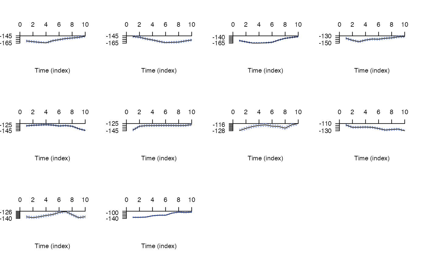
#### Example (6) Compare an automated vs. manual implementation of DC
## (A) Compare step-wise results for randomly select time steps
# Implement algorithm (using default calc_depth_error)
out_dc <- dc(
archival = depth,
bathy = dat_gebco,
save_record_spatial = NULL
)
#> flapper::dc() called (@ 2023-08-29 15:38:07)...
#> ... Setting up function...
#> 'calc_depth_error' function taken to be independent of depth.
#> ... Implementing calc_depth_error()...
#> ... Plotting movement time series (for each chunk)...
#> ... Implementing algorithm over time steps...
#> ... flapper::dc() call completed (@ 2023-08-29 15:38:12) after ~0.08 minutes.
# Compare results for randomly selected time steps to manual implementation
# ... with the same simple calc_depth_error model
pp <- graphics::par(mfrow = c(5, 2))
for (i in sample(1:nrow(depth), 5)) {
# Extract map created via dc()
raster::plot(out_dc$archive[[1]]$record[[i]]$spatial[[1]]$map_timestep)
# Compare to manual creation of map
raster::plot(dat_gebco >= depth$depth[i] - 2.5 & dat_gebco <= depth$depth[i] + 2.5)
}
 graphics::par(pp)
## (B) Compare the chunk-wise results and manual implementation
# Implement algorithm chunk-wise
out_dc <- dc(
archival = depth,
bathy = dat_gebco,
save_record_spatial = NULL,
split = 10L
)
#> flapper::dc() called (@ 2023-08-29 15:38:12)...
#> ... Setting up function...
#> 'calc_depth_error' function taken to be independent of depth.
#> ... Implementing calc_depth_error()...
#> ... Plotting movement time series (for each chunk)...
graphics::par(pp)
## (B) Compare the chunk-wise results and manual implementation
# Implement algorithm chunk-wise
out_dc <- dc(
archival = depth,
bathy = dat_gebco,
save_record_spatial = NULL,
split = 10L
)
#> flapper::dc() called (@ 2023-08-29 15:38:12)...
#> ... Setting up function...
#> 'calc_depth_error' function taken to be independent of depth.
#> ... Implementing calc_depth_error()...
#> ... Plotting movement time series (for each chunk)...
 #> ... Implementing algorithm over chunks...
#> ... flapper::dc() call completed (@ 2023-08-29 15:38:18) after ~0.09 minutes.
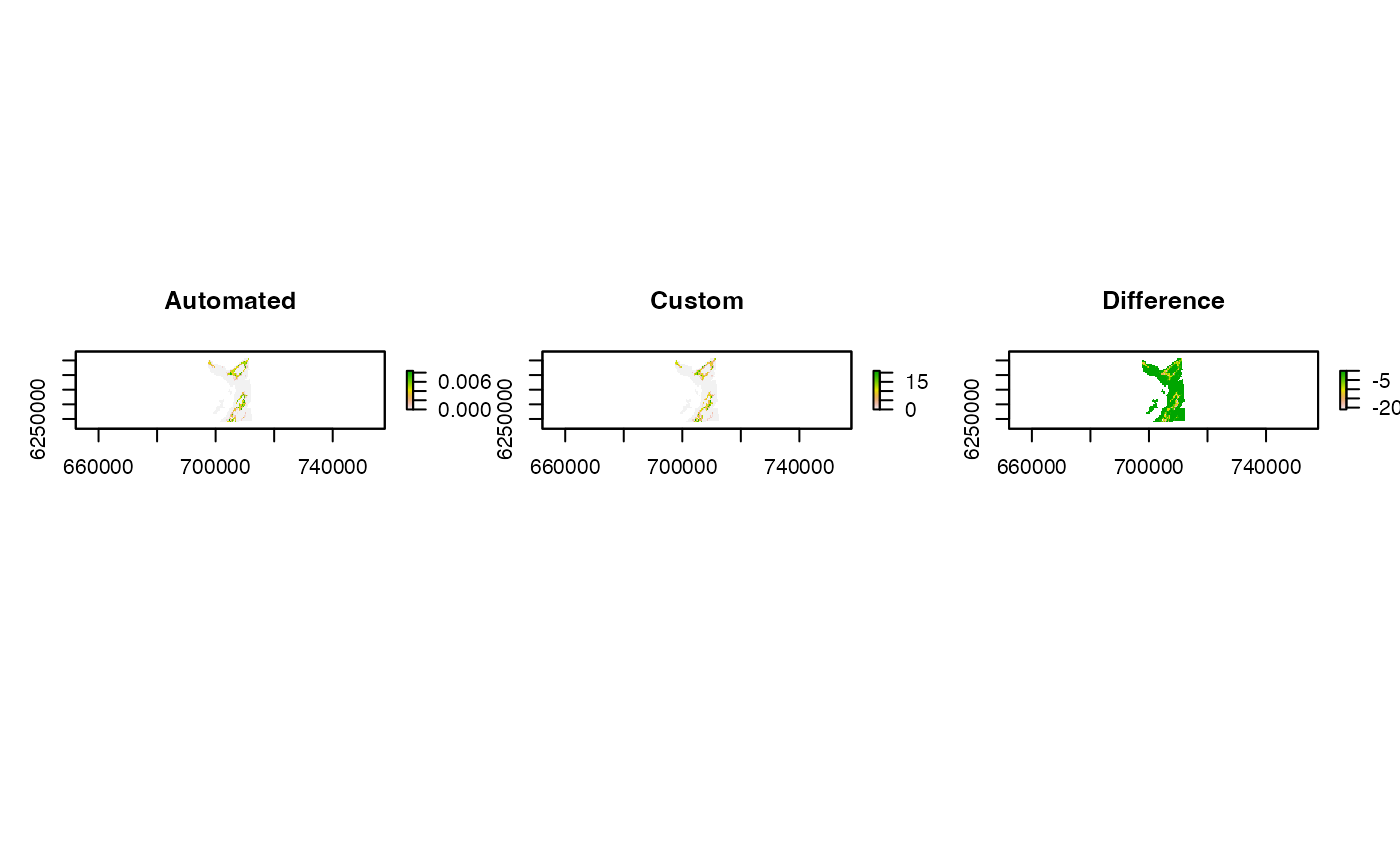
# Get overall map via acdc_simplify()
map_1 <- acdc_simplify(out_dc, type = "dc", mask = dat_gebco)$map
#> acdc_simplify() implemented for type = 'dc'.
# Get overall map via a simple custom approach
map_2 <- raster::setValues(dat_gebco, 0)
for (i in 1:nrow(depth)) {
map_2 <- map_2 + (dat_gebco >= depth$depth[i] - 2.5 & dat_gebco <= depth$depth[i] + 2.5)
}
map_2 <- raster::mask(map_2, dat_gebco)
# Show that the two overall maps are identical
pp <- par(mfrow = c(1, 3))
raster::plot(map_1, main = "Automated")
raster::plot(map_2, main = "Custom")
raster::plot(map_1 - map_2, main = "Difference")
#> ... Implementing algorithm over chunks...
#> ... flapper::dc() call completed (@ 2023-08-29 15:38:18) after ~0.09 minutes.
# Get overall map via acdc_simplify()
map_1 <- acdc_simplify(out_dc, type = "dc", mask = dat_gebco)$map
#> acdc_simplify() implemented for type = 'dc'.
# Get overall map via a simple custom approach
map_2 <- raster::setValues(dat_gebco, 0)
for (i in 1:nrow(depth)) {
map_2 <- map_2 + (dat_gebco >= depth$depth[i] - 2.5 & dat_gebco <= depth$depth[i] + 2.5)
}
map_2 <- raster::mask(map_2, dat_gebco)
# Show that the two overall maps are identical
pp <- par(mfrow = c(1, 3))
raster::plot(map_1, main = "Automated")
raster::plot(map_2, main = "Custom")
raster::plot(map_1 - map_2, main = "Difference")
 par(pp)