Plot time-specific maps from the AC/DC algorithm(s)
Source:R/acdc_analyse_record.R
acdc_plot_record.RdThis function is used to plot time-specific maps from the AC/DC algorithm(s). To implement the function, an acdc_record-class list from ac, dc or acdc plus acdc_simplify must be supplied, from which the results can be extracted and plotted for specified time steps. For each time step, the function extracts the necessary information; sets up a blank background plot using plot and pretty_axis and then adds requested spatial layers to this plot. Depending on user-inputs, this will usually show a cumulative map of expected time spent in different parts of the study area (from the start of the algorithm to each time point). Coastline, receivers and acoustic containers (if applicable) can be added and customised and the finalised plots can be returned or saved to file.
acdc_plot_record(
  record,
  type = c("map_cumulative", "map_timestep"),
  plot = 1,
  add_coastline = NULL,
  add_receivers = NULL,
  add_raster = list(col = rev(grDevices::terrain.colors(255))),
  add_containers = list(),
  add_additional = NULL,
  crop_spatial = FALSE,
  xlim = NULL,
  ylim = NULL,
  fix_zlim = FALSE,
  pretty_axis_args = list(side = 1:4, axis = list(list(), list(), list(labels = FALSE),
    list(labels = FALSE)), control_axis = list(las = TRUE), control_sci_notation =
    list(magnitude = 16L, digits = 0)),
  par_param = list(),
  png_param = list(),
  cl = NULL,
  varlist = NULL,
  verbose = TRUE,
  check = TRUE,
  ...
)
Arguments
- record
An
acdc_record-classobject.- type
A character that defines the plotted surface(s):
"map_cumulative"plots the cumulative surface and"map_timestep"plots time step-specific surfaces.- plot
An integer vector that defines the time steps for which to make plots. If
plot = NULL, the function will make a plot for all time steps for which the necessary information is available inrecord.- add_coastline
(optional) A named list of arguments, passed to
plot, to add a polygon (i.e., of the coastline), to the plot. If provided, this must contain an `x' element that contains the coastline as a spatial object (e.g., a SpatialPolygonsDataFrame: seedat_coastfor an example).- add_receivers
(optional) A named list of arguments, passed to
points, to add points (i.e., receivers) to the plot. If provided, this must contain an `x' element that is a SpatialPoints object that specifies receiver locations (in the same coordinate reference system as other spatial data).- add_raster
(optional) A named list of arguments, passed to
image.plot, to plot the RasterLayer of possible locations that is extracted fromrecord.- add_containers
(optional) For outputs from the AC* algorithms (
acoracdc),containersis a named list of arguments, passed toplot, to add the acoustic containers to the plot. If specified, the container that defines the boundaries of the individual's possible locations at each time step is drawn (i.e., `container_c` inacdc_record-classobjects).- add_additional
(optional) A stand-alone function, to be executed after the background plot has been made and any specified spatial layers have been added to this, to customise the result (see Examples).
- crop_spatial
A logical variable that defines whether or not to crop spatial data to lie within the axis limits.
- xlim, ylim, fix_zlim, pretty_axis_args
Axis control arguments.
xlimandylimcontrol the axis limits, following the rules of thelimargument inpretty_axis.fix_zlimis a logical input that defines whether or not to fix z axis limits across all plots (to facilitate comparisons), or a vector of two numbers that define a custom range for the z axis which is fixed across all plots.fix_zlim = FALSEproduces plots in which the z axis is allowed to vary flexibly between time units. Other axis options supported bypretty_axisare implemented by passing a named list of arguments to this function viapretty_axis_args.- par_param
(optional) A named list of arguments, passed to
par, to control the plotting window. This is executed before plotting is initiated and therefore affects all plots.- png_param
(optional) A named list of arguments, passed to
png, to save plots to file. If supplied, the plot for each time step is saved separately. The `filename' argument should be the directory in which plots are saved. Plots are then saved as "1.png", "2.png" and so on.- cl, varlist
(optional) Parallelisation options.
clis (a) a cluster object frommakeClusteror (b) an integer that defines the number of child processes.varlistis a character vector of variables for export (seecl_export). Exported variables must be located in the global environment. If a cluster is supplied, the connection to the cluster is closed within the function (seecl_stop). For further information, seecl_lapplyandflapper-tips-parallel. If supplied, the function loops over specified time steps in parallel to make plots. This is only implemented if plots are saved to file (i.e.,png_paramis supplied).- verbose
A logical variable that defines whether or not relay messages to the console to monitor function progress.
- check
A logical variable that defines whether or not to check user inputs to the function before its initiation.
- ...
Additional arguments, passed to
plot, to customise the blank background plot onto which spatial layers are added, such asxlab,ylabandmain.
Value
The function plots the results of the AC* algorithm(s) at specified time steps, with one plot per time step. Plots are saved to file if png_param is supplied.
See also
This function is typically used following calls to ac, dc or acdc and acdc_simplify.
Examples
#### Step (1): Implement AC/DC algorithm(s)
# ... see examples via ac(), dc() and acdc()
#### Step (2): Simplify outputs of the AC/DC algorithm(s)
dat_acdc <- acdc_simplify(dat_acdc)
#> acdc_simplify() implemented for type = 'acs'.
#### Example (1): The default options simply plot the first surface
acdc_plot_record(record = dat_acdc)
#> flapper::acdc_plot_record() called...
#> ... Checking function inputs...
#> ... Defining data for background plot...
#> ... Setting plotting window...
#> ... Making plots for each time step ...
#> Warning: Nothing to summarize if you provide a single RasterLayer; see cellStats
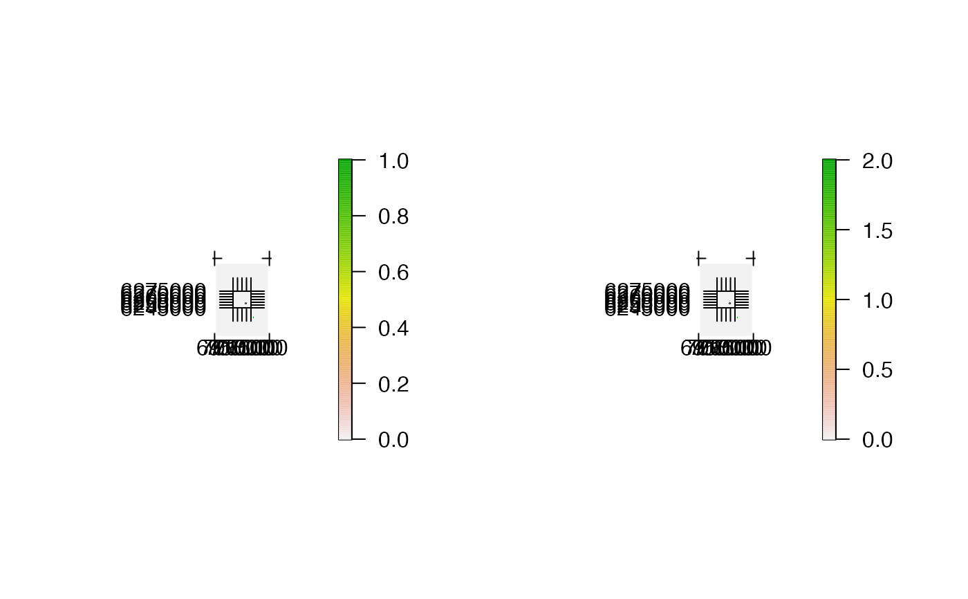
 #### Example (2): Define the number of plots to be produced and control the plotting window
acdc_plot_record(
record = dat_acdc,
plot = 1:2,
par_param = list(mfrow = c(1, 2), mar = c(8, 8, 8, 8))
)
#> flapper::acdc_plot_record() called...
#> ... Checking function inputs...
#> ... Defining data for background plot...
#> ... Setting plotting window...
#> ... Making plots for each time step ...
#> Warning: Nothing to summarize if you provide a single RasterLayer; see cellStats
#> Warning: Nothing to summarize if you provide a single RasterLayer; see cellStats
#### Example (2): Define the number of plots to be produced and control the plotting window
acdc_plot_record(
record = dat_acdc,
plot = 1:2,
par_param = list(mfrow = c(1, 2), mar = c(8, 8, 8, 8))
)
#> flapper::acdc_plot_record() called...
#> ... Checking function inputs...
#> ... Defining data for background plot...
#> ... Setting plotting window...
#> ... Making plots for each time step ...
#> Warning: Nothing to summarize if you provide a single RasterLayer; see cellStats
#> Warning: Nothing to summarize if you provide a single RasterLayer; see cellStats
 #### Example (3): Add and customise spatial information via add_* args
## Define a SpatialPoints object of receiver locations
proj_wgs84 <- sp::CRS(SRS_string = "EPSG:4326")
proj_utm <- sp::CRS(SRS_string = "EPSG:32629")
rsp <- sp::SpatialPoints(dat_moorings[, c("receiver_long", "receiver_lat")], proj_wgs84)
rsp <- sp::spTransform(rsp, proj_utm)
## Plot with receiver locations and coastline, customise the containers and the raster
acdc_plot_record(
record = dat_acdc,
add_coastline = list(x = dat_coast, col = "darkgreen"),
add_receivers = list(x = rsp, pch = 4, col = "royalblue"),
add_containers = list(col = "red"),
add_raster = list(col = rev(topo.colors(100)))
)
#> flapper::acdc_plot_record() called...
#> ... Checking function inputs...
#> ... Defining data for background plot...
#> ... Setting plotting window...
#> ... Making plots for each time step ...
#> Warning: Nothing to summarize if you provide a single RasterLayer; see cellStats
#### Example (4): Control axis properties
# ... via smallplot argument for raster, pretty_axis_args, xlim, ylim and fix_zlim
# ... set crop_spatial = TRUE to crop spatial data within adjusted limits
acdc_plot_record(
record = dat_acdc,
add_coastline = list(x = dat_coast, col = "darkgreen"),
add_receivers = list(x = rsp, pch = 4, col = "royalblue"),
add_containers = list(col = "red"),
add_raster = list(smallplot = c(0.85, 0.9, 0.25, 0.75)),
crop_spatial = TRUE,
pretty_axis_args = list(
side = 1:4,
control_sci_notation =
list(magnitude = 16L, digits = 0)
),
xlim = raster::extent(dat_coast)[1:2],
ylim = raster::extent(dat_coast)[3:4],
fix_zlim = c(0, 1)
)
#> flapper::acdc_plot_record() called...
#> ... Checking function inputs...
#> ... Defining data for background plot...
#> ... Setting plotting window...
#> ... Making plots for each time step ...
#> Warning: Nothing to summarize if you provide a single RasterLayer; see cellStats
#### Example (3): Add and customise spatial information via add_* args
## Define a SpatialPoints object of receiver locations
proj_wgs84 <- sp::CRS(SRS_string = "EPSG:4326")
proj_utm <- sp::CRS(SRS_string = "EPSG:32629")
rsp <- sp::SpatialPoints(dat_moorings[, c("receiver_long", "receiver_lat")], proj_wgs84)
rsp <- sp::spTransform(rsp, proj_utm)
## Plot with receiver locations and coastline, customise the containers and the raster
acdc_plot_record(
record = dat_acdc,
add_coastline = list(x = dat_coast, col = "darkgreen"),
add_receivers = list(x = rsp, pch = 4, col = "royalblue"),
add_containers = list(col = "red"),
add_raster = list(col = rev(topo.colors(100)))
)
#> flapper::acdc_plot_record() called...
#> ... Checking function inputs...
#> ... Defining data for background plot...
#> ... Setting plotting window...
#> ... Making plots for each time step ...
#> Warning: Nothing to summarize if you provide a single RasterLayer; see cellStats
#### Example (4): Control axis properties
# ... via smallplot argument for raster, pretty_axis_args, xlim, ylim and fix_zlim
# ... set crop_spatial = TRUE to crop spatial data within adjusted limits
acdc_plot_record(
record = dat_acdc,
add_coastline = list(x = dat_coast, col = "darkgreen"),
add_receivers = list(x = rsp, pch = 4, col = "royalblue"),
add_containers = list(col = "red"),
add_raster = list(smallplot = c(0.85, 0.9, 0.25, 0.75)),
crop_spatial = TRUE,
pretty_axis_args = list(
side = 1:4,
control_sci_notation =
list(magnitude = 16L, digits = 0)
),
xlim = raster::extent(dat_coast)[1:2],
ylim = raster::extent(dat_coast)[3:4],
fix_zlim = c(0, 1)
)
#> flapper::acdc_plot_record() called...
#> ... Checking function inputs...
#> ... Defining data for background plot...
#> ... Setting plotting window...
#> ... Making plots for each time step ...
#> Warning: Nothing to summarize if you provide a single RasterLayer; see cellStats
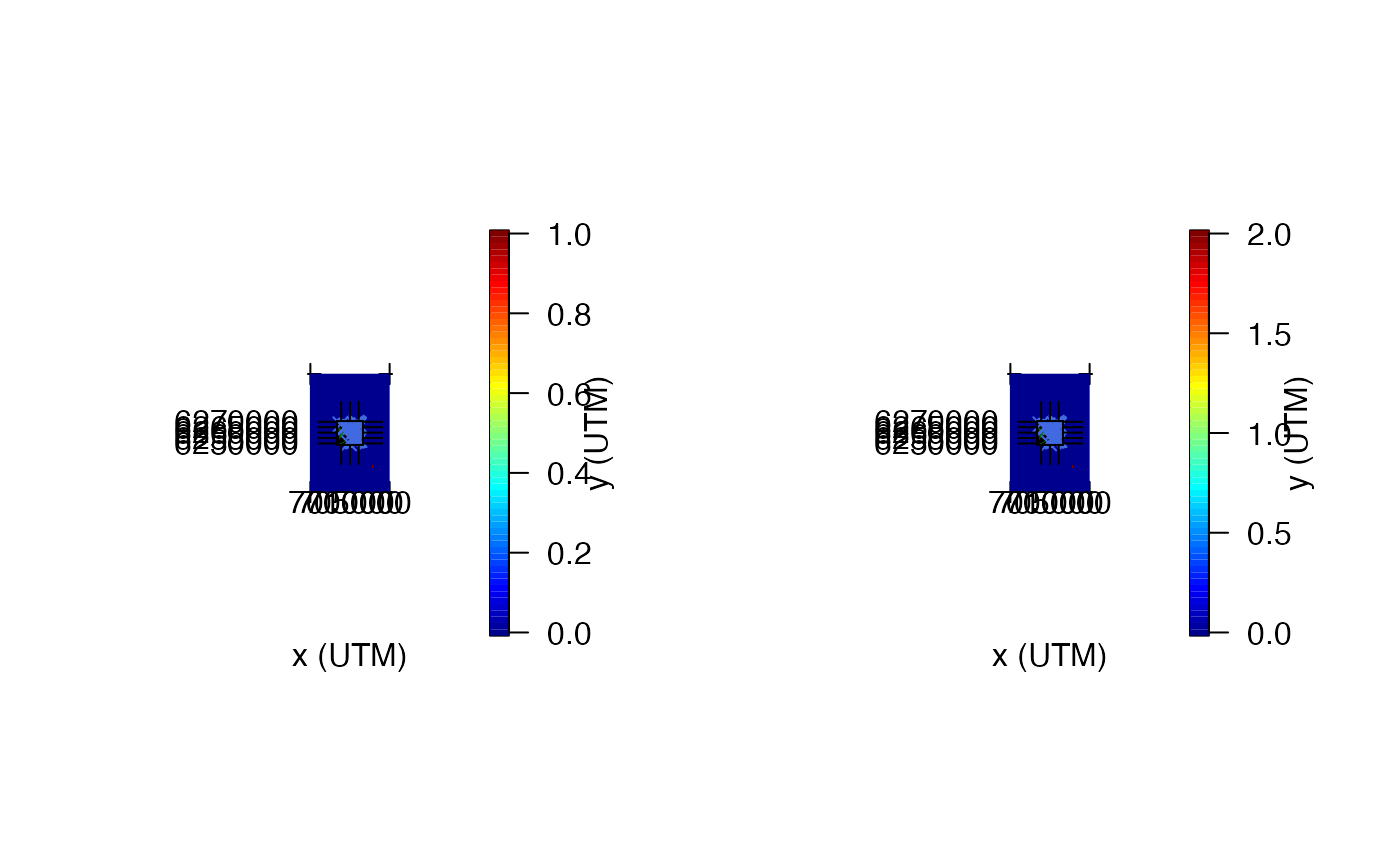
 #### Example (5): Modify each plot after it is produced via add_additional
# Specify a function to add titles to a plot
add_titles <- function() {
mtext(side = 1, "x (UTM)", line = 2)
mtext(side = 2, "y (UTM)", line = -8)
}
# Make plots with added titles
acdc_plot_record(
record = dat_acdc,
plot = 1:2,
par_param = list(mfrow = c(1, 2), mar = c(8, 8, 8, 8)),
add_coastline = list(x = dat_coast, col = "darkgreen"),
add_receivers = list(x = rsp, pch = 4, col = "royalblue"),
add_containers = list(col = "red"),
add_raster = list(),
crop_spatial = TRUE,
xlim = raster::extent(dat_coast)[1:2],
ylim = raster::extent(dat_coast)[3:4],
add_additional = add_titles
)
#> flapper::acdc_plot_record() called...
#> ... Checking function inputs...
#> ... Defining data for background plot...
#> ... Setting plotting window...
#> ... Making plots for each time step ...
#> Warning: Nothing to summarize if you provide a single RasterLayer; see cellStats
#> Warning: Nothing to summarize if you provide a single RasterLayer; see cellStats
#### Example (5): Modify each plot after it is produced via add_additional
# Specify a function to add titles to a plot
add_titles <- function() {
mtext(side = 1, "x (UTM)", line = 2)
mtext(side = 2, "y (UTM)", line = -8)
}
# Make plots with added titles
acdc_plot_record(
record = dat_acdc,
plot = 1:2,
par_param = list(mfrow = c(1, 2), mar = c(8, 8, 8, 8)),
add_coastline = list(x = dat_coast, col = "darkgreen"),
add_receivers = list(x = rsp, pch = 4, col = "royalblue"),
add_containers = list(col = "red"),
add_raster = list(),
crop_spatial = TRUE,
xlim = raster::extent(dat_coast)[1:2],
ylim = raster::extent(dat_coast)[3:4],
add_additional = add_titles
)
#> flapper::acdc_plot_record() called...
#> ... Checking function inputs...
#> ... Defining data for background plot...
#> ... Setting plotting window...
#> ... Making plots for each time step ...
#> Warning: Nothing to summarize if you provide a single RasterLayer; see cellStats
#> Warning: Nothing to summarize if you provide a single RasterLayer; see cellStats
 #### Example (6) Save plots via png_param
list.files(tempdir())
#> [1] "25" "28"
#> [3] "35" "ACDC_algorithm_demo.html"
#> [5] "acdc_log.txt" "css"
#> [7] "dot_acdc_log_1.txt" "dot_acdc_log_2.txt"
#> [9] "dot_acdc_log_3.txt" "dot_acdc_log_4.txt"
#> [11] "dot_acdc_log_5.txt" "downlit"
#> [13] "file1217f1b0b625c" "file1217f667087b8"
#> [15] "file1217f6772064" "file1217f67eddc54"
#> [17] "images" "js"
acdc_plot_record(
record = dat_acdc,
plot = 1:2,
png_param = list(filename = tempdir())
)
#> flapper::acdc_plot_record() called...
#> ... Checking function inputs...
#> '/' added to the directory inputted to the argument 'png_param$filename' ('/var/folders/nl/ygb3g6tj24z06jddbqqhj6hw0000gn/T//Rtmpwb5KFV').
#> ... Defining data for background plot...
#> ... Setting plotting window...
#> ... Making plots for each time step ...
#> Warning: Nothing to summarize if you provide a single RasterLayer; see cellStats
#> Warning: Nothing to summarize if you provide a single RasterLayer; see cellStats
list.files(tempdir())
#> [1] "1.png" "2.png"
#> [3] "25" "28"
#> [5] "35" "ACDC_algorithm_demo.html"
#> [7] "acdc_log.txt" "css"
#> [9] "dot_acdc_log_1.txt" "dot_acdc_log_2.txt"
#> [11] "dot_acdc_log_3.txt" "dot_acdc_log_4.txt"
#> [13] "dot_acdc_log_5.txt" "downlit"
#> [15] "file1217f1b0b625c" "file1217f667087b8"
#> [17] "file1217f6772064" "file1217f67eddc54"
#> [19] "images" "js"
#### Example (7) To plot the overall map, you can also just use a
# ... a raster plotting function like prettyGraphics::pretty_map()
ext <- update_extent(raster::extent(dat_coast), -1000)
prettyGraphics::pretty_map(
x = ext,
add_rasters = list(x = dat_acdc$map),
add_points = list(x = rsp, pch = "*", col = "red"),
add_polys = list(x = dat_coast, col = "lightgreen"),
crop_spatial = TRUE,
xlab = "Easting", ylab = "Northing"
)
#> Spatial layers do not have identical CRS strings
#> prettyGraphics::pretty_map() CRS taken as: 'NA'.
#### Example (6) Save plots via png_param
list.files(tempdir())
#> [1] "25" "28"
#> [3] "35" "ACDC_algorithm_demo.html"
#> [5] "acdc_log.txt" "css"
#> [7] "dot_acdc_log_1.txt" "dot_acdc_log_2.txt"
#> [9] "dot_acdc_log_3.txt" "dot_acdc_log_4.txt"
#> [11] "dot_acdc_log_5.txt" "downlit"
#> [13] "file1217f1b0b625c" "file1217f667087b8"
#> [15] "file1217f6772064" "file1217f67eddc54"
#> [17] "images" "js"
acdc_plot_record(
record = dat_acdc,
plot = 1:2,
png_param = list(filename = tempdir())
)
#> flapper::acdc_plot_record() called...
#> ... Checking function inputs...
#> '/' added to the directory inputted to the argument 'png_param$filename' ('/var/folders/nl/ygb3g6tj24z06jddbqqhj6hw0000gn/T//Rtmpwb5KFV').
#> ... Defining data for background plot...
#> ... Setting plotting window...
#> ... Making plots for each time step ...
#> Warning: Nothing to summarize if you provide a single RasterLayer; see cellStats
#> Warning: Nothing to summarize if you provide a single RasterLayer; see cellStats
list.files(tempdir())
#> [1] "1.png" "2.png"
#> [3] "25" "28"
#> [5] "35" "ACDC_algorithm_demo.html"
#> [7] "acdc_log.txt" "css"
#> [9] "dot_acdc_log_1.txt" "dot_acdc_log_2.txt"
#> [11] "dot_acdc_log_3.txt" "dot_acdc_log_4.txt"
#> [13] "dot_acdc_log_5.txt" "downlit"
#> [15] "file1217f1b0b625c" "file1217f667087b8"
#> [17] "file1217f6772064" "file1217f67eddc54"
#> [19] "images" "js"
#### Example (7) To plot the overall map, you can also just use a
# ... a raster plotting function like prettyGraphics::pretty_map()
ext <- update_extent(raster::extent(dat_coast), -1000)
prettyGraphics::pretty_map(
x = ext,
add_rasters = list(x = dat_acdc$map),
add_points = list(x = rsp, pch = "*", col = "red"),
add_polys = list(x = dat_coast, col = "lightgreen"),
crop_spatial = TRUE,
xlab = "Easting", ylab = "Northing"
)
#> Spatial layers do not have identical CRS strings
#> prettyGraphics::pretty_map() CRS taken as: 'NA'.