Process a kernel utilisation distribution around a barrier
Source:R/kud_tools.R
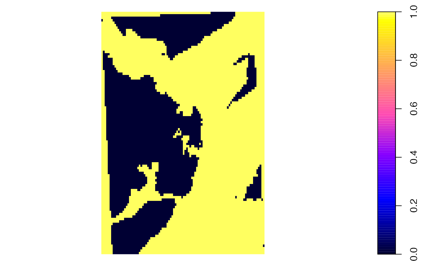
kud_around_coastline.RdGiven an animal movement path over a gridded surface, kud_around_coastline estimates a `raw' kernel utilisation distribution (from kernelUD) and then processes the distribution to account for barriers to movement, such as coastline. kud_around_coastline_fast is a bare-bones implementation of this function for iterative applications. To implement these functions, the movement path(s) should be supplied as a SpatialPointsDataFrame and the grid over which estimation is implemented as a SpatialPixelsDataFrame with values 0 and 1 defining unsuitable and suitable habitat respectively.
kud_around_coastline(xy, grid, ...)

kud_around_coastline_fast(xy, grid, ...)
Source
This forum is a useful resource: http://r-sig-geo.2731867.n2.nabble.com/Walruses-and-adehabitatHR-class-estUDm-exclusion-of-non-habitat-pixels-and-summary-over-all-animals-td6497315.html.
Arguments
- xy
A
SpatialPointsDataFrameobject that defines the movement path(s). This should contain a column that defines the individual ID(s) as a factor.kud_around_coastline_fastcan only handle one individual.- grid
A
SpatialPixelsDataFrameobject that defines the grid over which estimation is implemented and binary habitat suitability (0, unsuitable; or 1, suitable).- ...
Additional arguments passed to
kernelUD.
Value
kud_around_coastlinereturns an object of class `estUDm'. This is a list, with one component per animal, ofestUD-classobjects. The `h' slot of the output (output@h) has been modified so that the method (`meth') is given as `specified'.kud_around_coastline_fastreturns an object of class `RasterLayer'.
Details
Utilisation distributions (UDs) are bivariate probability distributions that describe the probability (density) of locating an individual in any given area at a randomly chosen time. These can be estimated using the kernelUD function. The algorithms implemented by kernelUD function can incorporate simple barriers, but restrictions on the shapes of barriers mean that in many real-world settings (e.g., in areas with complex coastline) barriers cannot be implemented. As a result, a pragmatic (if somewhat unsatisfactory) approach is to post-process the raw utilisation distribution by removing areas in which movement is impossible and then re-normalise the distribution (so that probabilities sum to one). These functions achieve this by implementing the estimation over a grid, which defines whether (1) or not (0) an area is `habitat'. After the estimation of the raw UD across the grid, probability density scores are combined (multiplied) with the habitat suitability score (0, 1) and then renormalised (by dividing by the total score across suitable areas).
To implement these routines, kud_around_coastline is typically the preferable option. kud_around_coastline is a bare-bones implementation of the routines within kud_around_coastline that has is designed to be (marginally) faster (e.g., for iterative applications). This function skips checks on user inputs, assuming that xy and grid have been correctly specified (as a SpatialPointsDataFrame for a specific individual and a SpatialPixelsDataFrame respectively), implements the estimation and returns a raster rather than an `estUDm' object (see Value).
Examples
#### Set up
## (1) Simulate path for which to compute UD
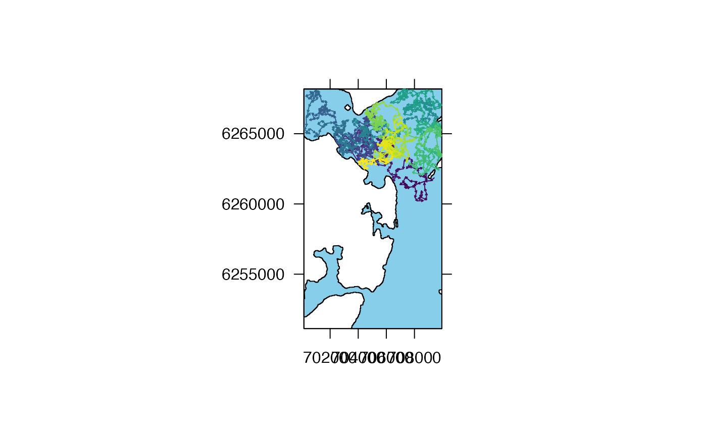
# Focus on a sample of the marine environment off Oban, West Scotland
sea <- invert_poly(dat_coast)
#> Warning: GEOS support is provided by the sf and terra packages among others
sea <- raster::crop(sea, update_extent(raster::extent(sea), x_shift = -2500))
prettyGraphics::pretty_map(add_polys = list(x = sea, col = "skyblue"))
#> prettyGraphics::pretty_map() CRS taken as: '+proj=utm +zone=29 +datum=WGS84 +units=m +no_defs'.
# Simulate path
n <- 1000
path_ls <- sim_path_sa(
n = n,
area = sea,
sim_step = function(...) stats::rgamma(1, shape = 20, scale = 20),
seed = 1,
plot = FALSE
)
#> flapper::sim_path_sa() called (@ 2023-08-29 15:42:35)...
#> ... Setting up simulation...
#> ... Simulating movement path...
#>
|
| | 0%
|
| | 1%
|
|= | 1%
|
|= | 2%
|
|== | 2%
|
|== | 3%
|
|== | 4%
|
|=== | 4%
|
|=== | 5%
|
|==== | 5%
|
|==== | 6%
|
|===== | 6%
|
|===== | 7%
|
|===== | 8%
|
|====== | 8%
|
|====== | 9%
|
|======= | 9%
|
|======= | 10%
|
|======= | 11%
|
|======== | 11%
|
|======== | 12%
|
|========= | 12%
|
|========= | 13%
|
|========= | 14%
|
|========== | 14%
|
|========== | 15%
|
|=========== | 15%
|
|=========== | 16%
|
|============ | 16%
|
|============ | 17%
|
|============ | 18%
|
|============= | 18%
|
|============= | 19%
|
|============== | 19%
|
|============== | 20%
|
|============== | 21%
|
|=============== | 21%
|
|=============== | 22%
|
|================ | 22%
|
|================ | 23%
|
|================ | 24%
|
|================= | 24%
|
|================= | 25%
|
|================== | 25%
|
|================== | 26%
|
|=================== | 26%
|
|=================== | 27%
|
|=================== | 28%
|
|==================== | 28%
|
|==================== | 29%
|
|===================== | 29%
|
|===================== | 30%
|
|===================== | 31%
|
|====================== | 31%
|
|====================== | 32%
|
|======================= | 32%
|
|======================= | 33%
|
|======================= | 34%
|
|======================== | 34%
|
|======================== | 35%
|
|========================= | 35%
|
|========================= | 36%
|
|========================== | 36%
|
|========================== | 37%
|
|========================== | 38%
|
|=========================== | 38%
|
|=========================== | 39%
|
|============================ | 39%
|
|============================ | 40%
|
|============================ | 41%
|
|============================= | 41%
|
|============================= | 42%
|
|============================== | 42%
|
|============================== | 43%
|
|============================== | 44%
|
|=============================== | 44%
|
|=============================== | 45%
|
|================================ | 45%
|
|================================ | 46%
|
|================================= | 46%
|
|================================= | 47%
|
|================================= | 48%
|
|================================== | 48%
|
|================================== | 49%
|
|=================================== | 49%
|
|=================================== | 50%
|
|=================================== | 51%
|
|==================================== | 51%
|
|==================================== | 52%
|
|===================================== | 52%
|
|===================================== | 53%
|
|===================================== | 54%
|
|====================================== | 54%
|
|====================================== | 55%
|
|======================================= | 55%
|
|======================================= | 56%
|
|======================================== | 56%
|
|======================================== | 57%
|
|======================================== | 58%
|
|========================================= | 58%
|
|========================================= | 59%
|
|========================================== | 59%
|
|========================================== | 60%
|
|========================================== | 61%
|
|=========================================== | 61%
|
|=========================================== | 62%
|
|============================================ | 62%
|
|============================================ | 63%
|
|============================================ | 64%
|
|============================================= | 64%
|
|============================================= | 65%
|
|============================================== | 65%
|
|============================================== | 66%
|
|=============================================== | 66%
|
|=============================================== | 67%
|
|=============================================== | 68%
|
|================================================ | 68%
|
|================================================ | 69%
|
|================================================= | 69%
|
|================================================= | 70%
|
|================================================= | 71%
|
|================================================== | 71%
|
|================================================== | 72%
|
|=================================================== | 72%
|
|=================================================== | 73%
|
|=================================================== | 74%
|
|==================================================== | 74%
|
|==================================================== | 75%
|
|===================================================== | 75%
|
|===================================================== | 76%
|
|====================================================== | 76%
|
|====================================================== | 77%
|
|====================================================== | 78%
|
|======================================================= | 78%
|
|======================================================= | 79%
|
|======================================================== | 79%
|
|======================================================== | 80%
|
|======================================================== | 81%
|
|========================================================= | 81%
|
|========================================================= | 82%
|
|========================================================== | 82%
|
|========================================================== | 83%
|
|========================================================== | 84%
|
|=========================================================== | 84%
|
|=========================================================== | 85%
|
|============================================================ | 85%
|
|============================================================ | 86%
|
|============================================================= | 86%
|
|============================================================= | 87%
|
|============================================================= | 88%
|
|============================================================== | 88%
|
|============================================================== | 89%
|
|=============================================================== | 89%
|
|=============================================================== | 90%
|
|=============================================================== | 91%
|
|================================================================ | 91%
|
|================================================================ | 92%
|
|================================================================= | 92%
|
|================================================================= | 93%
|
|================================================================= | 94%
|
|================================================================== | 94%
|
|================================================================== | 95%
|
|=================================================================== | 95%
|
|=================================================================== | 96%
|
|==================================================================== | 96%
|
|==================================================================== | 97%
|
|==================================================================== | 98%
|
|===================================================================== | 98%
|
|===================================================================== | 99%
|
|======================================================================| 99%
|
|======================================================================| 100%... flapper::sim_path_sa() call completed (@ 2023-08-29 15:42:36) after ~0.01 minutes.
prettyGraphics::add_sp_path(path_ls$xy_mat,
col = viridis::viridis(n),
length = 0.02
)
 ## (2) Define path as a SpatialPointsDataFrame (SpatialPoints is not allowed)
path <- sp::SpatialPointsDataFrame(
path_ls$xy_mat,
data = data.frame(ID = factor(rep(1, nrow(path_ls$xy_mat)))),
proj4string = raster::crs(dat_coast)
)
## (3) Define grid over which to implement estimation
# ... The grid needs to be sufficiently small to capture the coastline
# ... reasonably while being large enough to enable calculation
# ... of the home range.
r <- raster::raster(raster::extent(dat_coast), nrows = 100, ncols = 100)
raster::values(r) <- 0
r <- raster::mask(r, dat_coast, updatevalue = 1)
habitat <- methods::as(r, "SpatialPixelsDataFrame")
sp::plot(habitat)
 #### Example (1) Implement estimation and processing
## Estimate raw UD
ud_raw <- adehabitatHR::kernelUD(xy = path, grid = habitat)
# Object is of class estUDm, which is a list of estUD objects
# The outputs for each animal can be accessed by indexing
ud_raw[[1]]
#> Object of class "SpatialPixelsDataFrame" (package sp):
#>
#> Grid parameters:
#> cellcentre.offset cellsize cells.dim
#> Var2 697711.7 148.1125 100
#> Var1 6248737.3 220.5348 100
#>
#> Variables measured:
#> ud
#> 1 0
#> 2 0
#> 3 0
#> 4 0
#> 5 0
#> 6 0
#> ...
#>
# Check smoothing parameters
ud_raw[[1]]@h
#> $h
#> [1] 632.7372
#>
#> $meth
#> [1] "href"
#>
## Estimate raw UD and post-process
ud_pro <- kud_around_coastline(xy = path, grid = habitat)
# The same type of object is returned
ud_pro[[1]]
#> Object of class "SpatialPixelsDataFrame" (package sp):
#>
#> Grid parameters:
#> cellcentre.offset cellsize cells.dim
#> Var2 697711.7 148.1125 100
#> Var1 6248737.3 220.5348 100
#>
#> Variables measured:
#> ud
#> 1 0.000000e+00
#> 2 0.000000e+00
#> 3 0.000000e+00
#> 4 0.000000e+00
#> 5 0.000000e+00
#> 6 2.610702e-12
#> ...
#>
# Smoothing parameters have been modified
ud_pro[[1]]@h
#> $h
#> [1] 0
#>
#> $meth
#> [1] "specified"
#>
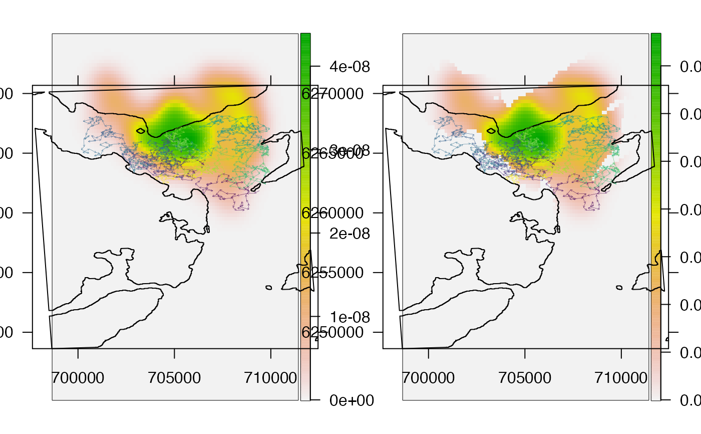
## Compare plots
# ... Notice that the processed version doesn't 'bleed' onto land
# ... and the scale differs due to the re-normalisation
ud_raw_r <- raster::raster(ud_raw[[1]])
ud_pro_r <- raster::raster(ud_pro[[1]])
pp <- graphics::par(mfrow = c(1, 2))
prettyGraphics::pretty_map(
add_rasters = list(x = ud_raw_r),
add_polys = list(x = dat_coast),
add_paths = list(
x = path,
col = viridis::viridis(n),
lwd = 0.25,
length = 0.02
)
)
#> Spatial layers do not have identical CRS strings
#> prettyGraphics::pretty_map() CRS taken as: '+proj=utm +zone=29 +datum=WGS84 +units=m +no_defs'.
prettyGraphics::pretty_map(
add_rasters = list(x = ud_pro_r),
add_polys = list(x = dat_coast),
add_paths = list(
x = path,
col = viridis::viridis(n),
lwd = 0.25,
length = 0.02
)
)
#> Spatial layers do not have identical CRS strings
#> prettyGraphics::pretty_map() CRS taken as: '+proj=utm +zone=29 +datum=WGS84 +units=m +no_defs'.
 graphics::par(pp)
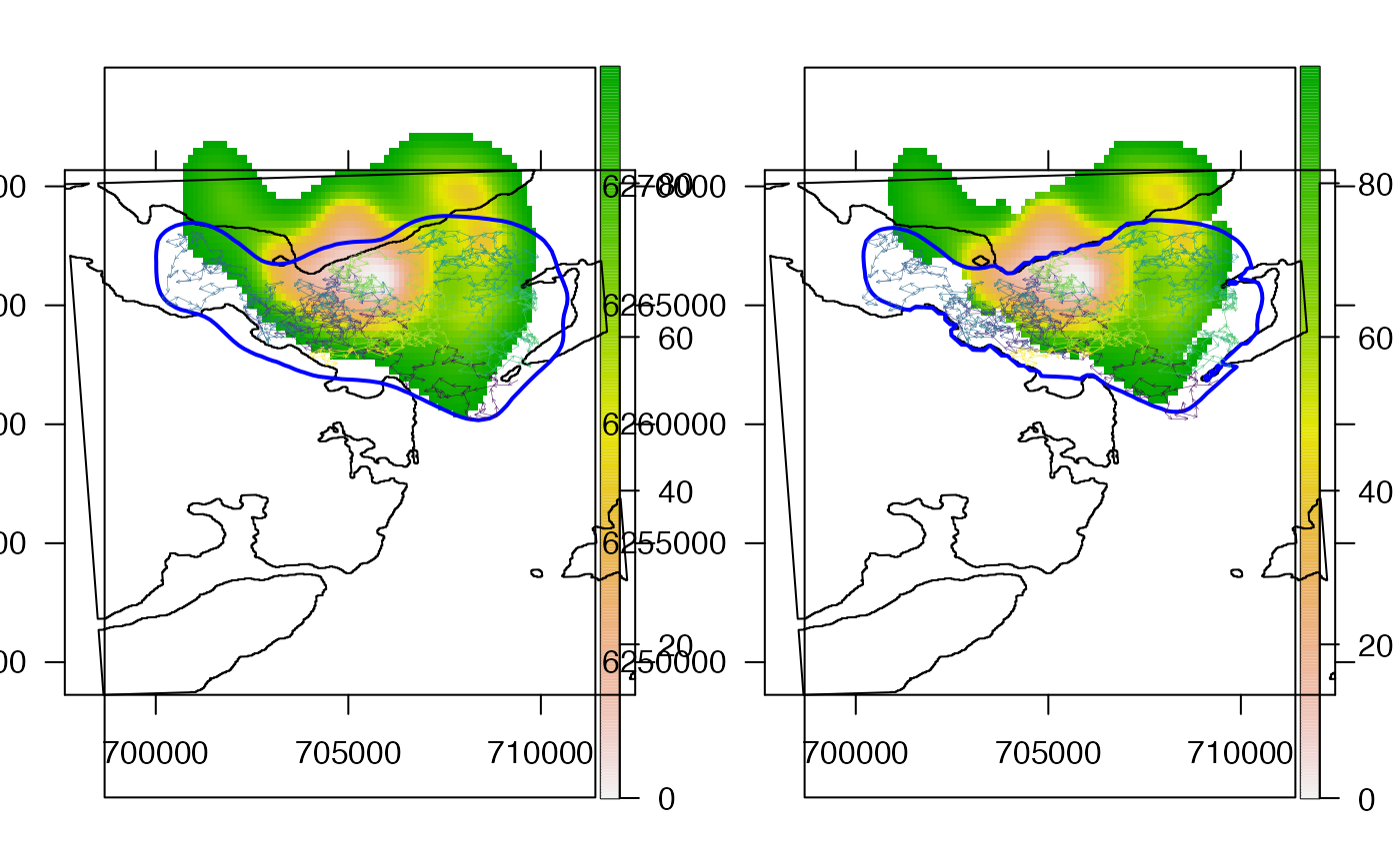
#### Further analysis can be implemented as usual
# For example we can compute the home range contours from the UD
# ... using adehabitatHR::getvolumeUD(). In practice, this converts from the
# ... probability density scale to a more intuitive % home range scale.
# Get volume
vol_raw <- adehabitatHR::getvolumeUD(ud_raw, standardize = TRUE)
vol_pro <- adehabitatHR::getvolumeUD(ud_pro, standardize = TRUE)
# Get contours
ver_raw <- adehabitatHR::getverticeshr(ud_raw[[1]], standardize = TRUE)
ver_pro <- adehabitatHR::getverticeshr(ud_pro[[1]], standardize = TRUE)
# Rasterise
vol_raw_r <- raster::raster(vol_raw[[1]])
vol_pro_r <- raster::raster(vol_pro[[1]])
# For neatness on the plot, it is convenient to exclude areas beyond 95 %
vol_raw_r[vol_raw_r[] > 95] <- NA
vol_pro_r[vol_pro_r[] > 95] <- NA
# Plot
pp <- graphics::par(mfrow = c(1, 2))
prettyGraphics::pretty_map(
add_rasters = list(x = vol_raw_r),
add_polys = list(
list(x = dat_coast),
list(
x = ver_raw,
border = "blue",
lwd = 2
)
),
add_paths = list(
x = path,
col = viridis::viridis(n),
lwd = 0.25,
length = 0.02
)
)
#> Spatial layers do not have identical CRS strings
#> prettyGraphics::pretty_map() CRS taken as: '+proj=utm +zone=29 +datum=WGS84 +units=m +no_defs'.
prettyGraphics::pretty_map(
add_rasters = list(x = vol_pro_r),
add_polys = list(
list(x = dat_coast),
list(
x = ver_pro,
border = "blue",
lwd = 2
)
),
add_paths = list(
x = path,
col = viridis::viridis(n),
lwd = 0.25,
length = 0.02
)
)
#> Spatial layers do not have identical CRS strings
#> prettyGraphics::pretty_map() CRS taken as: '+proj=utm +zone=29 +datum=WGS84 +units=m +no_defs'.
 graphics::par(pp)