This function compares Euclidean distances to shortest distances for randomly sampled pairs of points across a raster.
lcp_comp(
  surface,
  barrier = NULL,
  distance = NULL,
  interval = raster::res(surface)[1],
  mobility = NULL,
  n = 10L,
  n_max = n,
  graph = NULL,
  ...,
  cl = NULL,
  varlist = NULL,
  verbose = TRUE
)
Arguments
- surface
A
rasterfrom which to sample locations and calculate distances. Thesurfacemust be planar with units of metres in x, y and z directions. Theresolutionmust be the same in both x and y directions (seelcp_over_surface). If applicable, thesurfaceshould be masked bybarrier(seemask_io) prior to implementation of this function.- barrier
(optional) A simple features geometry that defines a barrier (see
segments_cross_barrier). If supplied, the function determines whether or not each sampled pair of coordinates crosses the barrier.- distance
A numeric vector of distances. If supplied, for each distance,
nlocation pairs that are that approximately that distance apart (seeinterval) are sampled and, for each pair, Euclidean and shortest distances are calculated. If supplied,mobilityshould not be supplied (see below).- interval
If
distanceis supplied,intervalis a number that defines the range of distances around each distance that are admissible. For example, ifdistance = 50(m) andinterval = 5,nlocation pairs that are within 45--55 m of each other are sampled.- mobility
(optional) A number that defines the maximum distance between sampled locations. If supplied,
nlocations are sampled; the Euclidean distances between all combinations of locations are calculated; and for the location pairs for which the Euclidean distance is less thanmobility(up to a maximum ofn_maxpairs), shortest distances are calculated. This method is potentially fast thedistance-vector-based method that is implemented isdistanceis supplied, but the final number of locations cannot be predetermined. If supplied,distanceshould not be supplied (see above).- n
An integer that defines (a) the number of location pairs for each
distanceor (b) the initial number of sampled locations ifmobilityis supplied.- n_max
If
mobilityis supplied,n_maxis an integer that defines the maximum number of location pairs for which shortest distances are calculated.- graph
(optional) A graph object that defines cell nodes and edge costs for connected cells within the surface (see
lcp_graph_surface). This is used for shortest-distance calculations.- ...
Additional arguments passed to
get_distance_pairfor shortest-distance calculations (algorithm,constantand/orallcores).- cl, varlist
(optional) Parallelisation options for distance-based location sampling (i.e., if
distance != NULL).clis (a) a cluster object frommakeClusteror (b) an integer that defines the number of child processes.varlistis a character vector of variables for export (seecl_export). Exported variables must be located in the global environment. If a cluster is supplied, the connection to the cluster is closed within the function (seecl_stop). For further information, seecl_lapplyandflapper-tips-parallel.- verbose
A logical input that defines whether or not to print messages to the console to monitor function progress.
Value
The function returns a dataframe with sampled location pairs and the Euclidean and shortest distances between them. This contains the following columns:
index -- A number that defines the row.
id -- If
distanceis specified,idis number that defines the sample (from1:nfor eachdistance).cell_x0, cell_y0, cell_x1, cell_y1 -- Numbers that define the coordinates of sampled locations.
cell_id0, cell_id1 -- Integers that define the cell IDs for sampled locations.
dist_sim -- If
distanceis specified,dist_simis a number that defines the specified distance.dist_euclid -- A number that defines the Euclidean distance from
(cell_x0, cell_y0)to(cell_x1, cell_y1).dist_lcp -- A number that defines the shortest distance from
(cell_x0, cell_y0)to(cell_x1, cell_y1).barrier -- If applicable,
barrieris factor that defines whether ("1") or not ("0") the Euclidean line connecting(cell_x0, cell_y0)and(cell_x1, cell_y1)crosses thebarrier.
Details
This function was motivated by the need to determine the extent to which Euclidean distances are a suitable approximation of shortest distances in movement models for benthic animals.
To address this issue, this function samples multiple pairs of points on a raster (surface) and compares the Euclidean and shortest distances between sampled locations.
Two sampling methods are implemented. The first method (implemented if distance is supplied), samples n pairs of points for each distance that are approximately that distance apart. (Sampling across a grid is approximate because grid resolution is finite. The approximation is controlled by the interval parameter.) The advantage of this method is that the number of sampled location pairs for which Euclidean and shortest distances are compared is predetermined (by n), but the method can be slow if n is large. The second method (implemented if mobility is supplied), simply samples n locations and calculates the Euclidean distances between all combinations of sampled locations. Any location pairs that are more than mobility apart are then dropped and for the remaining location pairs (up to a maximum of n_max randomly sampled pairs) shortest distances are calculated. A potential advantage of this method is speed, but the number of location pairs below mobility for which Euclidean and shortest distances can be compared is not predetermined.
Regardless of sampling method, the expectation for the analysis is that at short Euclidean distances, Euclidean distances are likely to approximate shortest distances well (unless there is a barrier, such as the coastline, in the way). At longer Euclidean distances, shortest distances are likely to become much longer than Euclidean distances. For some movement frameworks, especially the particle filtering (pf) and processing (pf_simplify) routines in flapper, the Euclidean distance at which the shortest distances start to exceed the distance that an animal could move (over some time interval of interest) is an important parameter (termed calc_distance_limit in pf_simplify). For sampled locations that are a Euclidean distance less than this threshold apart, it is reasonable to assume that there exists a `valid' shortest path over the surface, given the animal's mobility, without having to calculate that path; for sampled locations that are a Euclidean distance more than this threshold apart, this assumption is not valid. For areas with a clear-cut threshold, for Euclidean-based sampling frameworks (see pf), it may be reasonable to reduce the animal's mobility to the threshold value to account for this difference; in other cases, it may be necessary to compute shortest distances for potentially problematic locations. Either way, an understanding of the extent to which Euclidean distances effectively approximate shortest distances at spatial scales relevant to an animal can help to minimise the number of shortest-distance calculations that are required within a movement modelling framework (which are much more computationally demanding than Euclidean-based calculations).
Examples
#### Load packages
require(prettyGraphics)
#> Loading required package: prettyGraphics
#>
#> Attaching package: ‘prettyGraphics’
#> The following object is masked from ‘package:flapper’:
#>
#> dat_gebco
#### Define surface for examples
# We will focus on a relatively small area for speed
# The raster resolution should be equal in x and y directions
bathy <- flapper::dat_gebco
boundaries <- raster::extent(700652.2, 708401.2, 6262905, 6270179)
blank <- raster::raster(boundaries, res = c(5, 5))
bathy <- raster::resample(bathy, blank)
bathy <- mask_io(bathy, flapper::dat_coast, mask_inside = TRUE)
#> Warning: GEOS support is provided by the sf and terra packages among others
#> Warning: spgeom1 and spgeom2 have different proj4 strings
# raster::plot(bathy)
# raster::lines(dat_coast)
#### Define barrier to movement
coastline <- raster::crop(dat_coast, raster::extent(bathy))
coastline <- sf::st_as_sf(coastline)
#### Define graph for shortest-distance calculations
bathy_costs <- lcp_costs(bathy) # ~0.38 mins
#> flapper::lcp_costs() called (@ 2023-08-29 15:42:40)...
#> ... Defining transition matrices...
#> Warning: transition function gives negative values
#> ... Calculating distance matrices...
#> ... Assembling LCP costs...
#> ... flapper::lcp_costs() call completed (@ 2023-08-29 15:42:59) after ~0.31 minutes.
bathy_graph <- lcp_graph_surface(bathy, bathy_costs$dist_total) # ~0.26 mins
#> flapper::lcp_graph_surface() called (@ 2023-08-29 15:42:59)...
#> ... Defining nodes, edges and costs to make graph...
#> ... Constructing graph object...
#> ... flapper::lcp_graph_surface() call completed (@ 2023-08-29 15:43:08) after ~0.16 minutes.
#### Example (1): Distance-vector-based implementation
## Implement function
out_1 <- lcp_comp(
surface = bathy,
distance = c(50, 100),
graph = bathy_graph,
barrier = coastline
)
#> flapper::lcp_comp() called (@ 2023-08-29 15:43:08)...
#> ... Defining parameters...
#> ... Sampling n location pairs for each distance value...
#> ... ... Sampling for distance = 50...
#> ... ... ... Sampling starting locations...
#> ... ... ... Sampling ending locations...
#> ... ... Sampling for distance = 100...
#> ... ... ... Sampling starting locations...
#> ... ... ... Sampling ending locations...
#> ... Processing samples...
#> ... Determining barrier overlaps...
#> ... Implementing shortest-distance calculations...
#> ... ... Calculating shortest-distances via cppRouting::get_distance_pair() for 20 location pair(s) ...
#> ... Cleaning results...
#> ... flapper::lcp_comp() call completed (@ 2023-08-29 15:43:16) after ~0.13 minutes.
## Examine outputs
# The function returns a dataframe
utils::str(out_1)
#> 'data.frame': 20 obs. of 12 variables:
#> $ index : int 1 2 3 4 5 6 7 8 9 10 ...
#> $ id : int 1 2 3 4 5 6 7 8 9 10 ...
#> $ cell_x0 : num 701520 701955 705210 707355 703900 ...
#> $ cell_y0 : num 6265956 6267946 6265682 6266712 6263782 ...
#> $ cell_x1 : num 701475 701965 705210 707340 703945 ...
#> $ cell_y1 : num 6265926 6267996 6265632 6266666 6263762 ...
#> $ cell_id0 : num 1308374 691561 1394362 1075491 1983100 ...
#> $ cell_id1 : num 1317665 676063 1409862 1089438 1989309 ...
#> $ dist_sim : num 50 50 50 50 50 50 50 50 50 50 ...
#> $ dist_euclid: num 54.1 51 50 47.4 49.2 ...
#> $ dist_lcp : num 57.4 54.2 50 51.2 53.3 ...
#> $ barrier : Factor w/ 2 levels "0","1": 1 1 1 1 1 1 1 1 1 1 ...
## Visualise sampled locations on map
raster::plot(bathy)
raster::lines(dat_coast)
invisible(lapply(split(out_1, seq_len(nrow(out_1))), function(d) {
arrows(
x0 = d$cell_x0, y0 = d$cell_y0,
x1 = d$cell_x1, y1 = d$cell_y1, length = 0.01, lwd = 2
)
}))
 ## Compare simulated, Euclidean and shortest distances
pp <- graphics::par(mfrow = c(1, 2))
pretty_plot(out_1$dist_sim, out_1$dist_euclid,
xlab = "Distance (simulated) [m]",
ylab = "Distance (Euclidean)[m]"
)
graphics::abline(0, 1)
pretty_plot(out_1$dist_euclid, out_1$dist_lcp,
xlab = "Distance (Euclidean) [m]",
ylab = "Distance (shortest) [m]"
)
graphics::abline(0, 1)
## Compare simulated, Euclidean and shortest distances
pp <- graphics::par(mfrow = c(1, 2))
pretty_plot(out_1$dist_sim, out_1$dist_euclid,
xlab = "Distance (simulated) [m]",
ylab = "Distance (Euclidean)[m]"
)
graphics::abline(0, 1)
pretty_plot(out_1$dist_euclid, out_1$dist_lcp,
xlab = "Distance (Euclidean) [m]",
ylab = "Distance (shortest) [m]"
)
graphics::abline(0, 1)
 graphics::par(pp)
#### Example (2): Distance-vector-based implementation in parallel
out_2 <- lcp_comp(
surface = bathy,
distance = c(50, 100),
graph = bathy_graph,
barrier = coastline,
cl = parallel::makeCluster(2L)
)
#> flapper::lcp_comp() called (@ 2023-08-29 15:43:16)...
#> ... Defining parameters...
#> ... Sampling n location pairs for each distance value...
#> ... Processing samples...
#> ... Determining barrier overlaps...
#> ... Implementing shortest-distance calculations...
#> ... ... Calculating shortest-distances via cppRouting::get_distance_pair() for 20 location pair(s) ...
#> ... Cleaning results...
#> ... flapper::lcp_comp() call completed (@ 2023-08-29 15:43:27) after ~0.18 minutes.
#### Example (3): Mobility-based implementation
## Implement function for mobility = 500
mob <- 500
out_3 <- lcp_comp(
surface = bathy,
mobility = mob,
n = 1000,
graph = bathy_graph,
barrier = coastline
)
#> flapper::lcp_comp() called (@ 2023-08-29 15:43:27)...
#> ... Defining parameters...
#> ... Sampling n locations...
#> ... Calculating Euclidean distances between sampled locations...
#> ... Filtering by mobility...
#> ... Processing samples...
#> ... Determining barrier overlaps...
#> ... Implementing shortest-distance calculations...
#> ... ... Calculating shortest-distances via cppRouting::get_distance_pair() for 1000 location pair(s) ...
#> ... Cleaning results...
#> ... flapper::lcp_comp() call completed (@ 2023-08-29 15:43:29) after ~0.03 minutes.
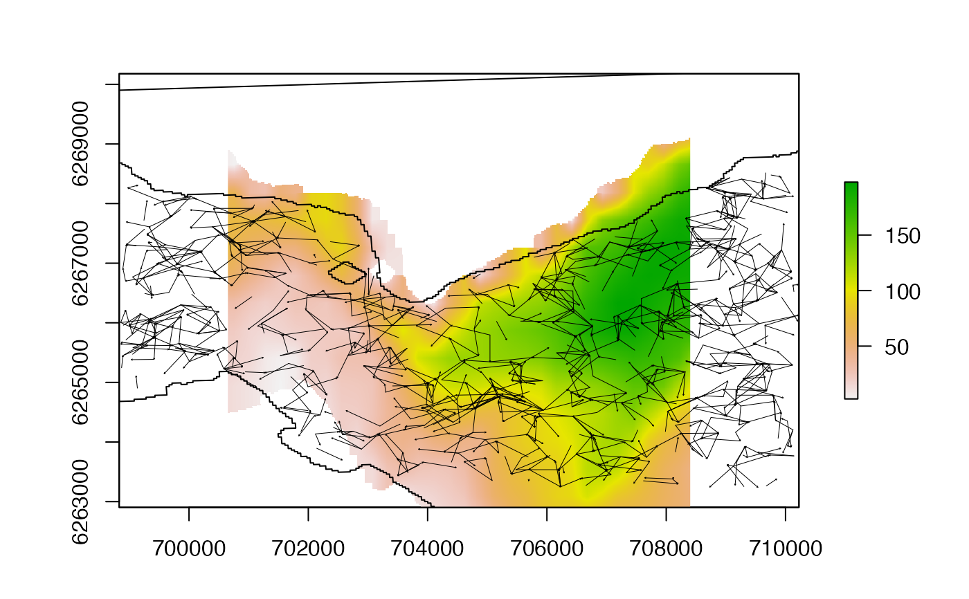
## Visualise sampled locations on map
raster::plot(bathy)
raster::lines(dat_coast)
invisible(lapply(split(out_3, seq_len(nrow(out_3))), function(d) {
arrows(
x0 = d$cell_x0, y0 = d$cell_y0,
x1 = d$cell_x1, y1 = d$cell_y1, length = 0.01, lwd = 0.5
)
}))
graphics::par(pp)
#### Example (2): Distance-vector-based implementation in parallel
out_2 <- lcp_comp(
surface = bathy,
distance = c(50, 100),
graph = bathy_graph,
barrier = coastline,
cl = parallel::makeCluster(2L)
)
#> flapper::lcp_comp() called (@ 2023-08-29 15:43:16)...
#> ... Defining parameters...
#> ... Sampling n location pairs for each distance value...
#> ... Processing samples...
#> ... Determining barrier overlaps...
#> ... Implementing shortest-distance calculations...
#> ... ... Calculating shortest-distances via cppRouting::get_distance_pair() for 20 location pair(s) ...
#> ... Cleaning results...
#> ... flapper::lcp_comp() call completed (@ 2023-08-29 15:43:27) after ~0.18 minutes.
#### Example (3): Mobility-based implementation
## Implement function for mobility = 500
mob <- 500
out_3 <- lcp_comp(
surface = bathy,
mobility = mob,
n = 1000,
graph = bathy_graph,
barrier = coastline
)
#> flapper::lcp_comp() called (@ 2023-08-29 15:43:27)...
#> ... Defining parameters...
#> ... Sampling n locations...
#> ... Calculating Euclidean distances between sampled locations...
#> ... Filtering by mobility...
#> ... Processing samples...
#> ... Determining barrier overlaps...
#> ... Implementing shortest-distance calculations...
#> ... ... Calculating shortest-distances via cppRouting::get_distance_pair() for 1000 location pair(s) ...
#> ... Cleaning results...
#> ... flapper::lcp_comp() call completed (@ 2023-08-29 15:43:29) after ~0.03 minutes.
## Visualise sampled locations on map
raster::plot(bathy)
raster::lines(dat_coast)
invisible(lapply(split(out_3, seq_len(nrow(out_3))), function(d) {
arrows(
x0 = d$cell_x0, y0 = d$cell_y0,
x1 = d$cell_x1, y1 = d$cell_y1, length = 0.01, lwd = 0.5
)
}))
 ## Compare Euclidean and shortest distances
# Extract the data for the paths that do not versus do cross a barrier
out_3_barrier0 <- out_3[out_3$barrier == 0, ]
out_3_barrier1 <- out_3[out_3$barrier == 1, ]
# Set up plotting window
pp <- graphics::par(mfrow = c(1, 2), oma = c(3, 3, 3, 3), mar = c(4, 4, 4, 4))
# Results for paths that do not cross a barrier
# ... Visualisation
pretty_plot(out_3_barrier0$dist_euclid, out_3_barrier0$dist_lcp,
xlab = "Distance (Euclidean) [m]",
ylab = "Distance (shortest) [m]",
pch = "."
)
graphics::abline(0, 1, col = "red")
graphics::abline(h = mob, col = "royalblue", lty = 3)
# ... Euclidean distance parameter at which mobility is exceeded
limit0 <- min(out_3_barrier0$dist_euclid[out_3_barrier0$dist_lcp > mob])
limit0
#> [1] 464.8656
graphics::abline(v = limit0, col = "royalblue", lty = 3)
# Results for paths that cross a barrier
# ... Visualisation
pretty_plot(out_3_barrier1$dist_euclid, out_3_barrier1$dist_lcp,
xlab = "Distance (Euclidean) [m]",
ylab = "Distance (shortest) [m]",
pch = "."
)
graphics::abline(0, 1, col = "red")
graphics::abline(h = mob, col = "royalblue", lty = 3)
# ... Euclidean distance parameter at which mobility is exceeded
limit1 <-
min(out_3_barrier1$dist_euclid[out_3_barrier1$dist_lcp > mob])
limit1
#> [1] 466.1545
graphics::abline(v = limit1, col = "royalblue", lty = 3)
## Compare Euclidean and shortest distances
# Extract the data for the paths that do not versus do cross a barrier
out_3_barrier0 <- out_3[out_3$barrier == 0, ]
out_3_barrier1 <- out_3[out_3$barrier == 1, ]
# Set up plotting window
pp <- graphics::par(mfrow = c(1, 2), oma = c(3, 3, 3, 3), mar = c(4, 4, 4, 4))
# Results for paths that do not cross a barrier
# ... Visualisation
pretty_plot(out_3_barrier0$dist_euclid, out_3_barrier0$dist_lcp,
xlab = "Distance (Euclidean) [m]",
ylab = "Distance (shortest) [m]",
pch = "."
)
graphics::abline(0, 1, col = "red")
graphics::abline(h = mob, col = "royalblue", lty = 3)
# ... Euclidean distance parameter at which mobility is exceeded
limit0 <- min(out_3_barrier0$dist_euclid[out_3_barrier0$dist_lcp > mob])
limit0
#> [1] 464.8656
graphics::abline(v = limit0, col = "royalblue", lty = 3)
# Results for paths that cross a barrier
# ... Visualisation
pretty_plot(out_3_barrier1$dist_euclid, out_3_barrier1$dist_lcp,
xlab = "Distance (Euclidean) [m]",
ylab = "Distance (shortest) [m]",
pch = "."
)
graphics::abline(0, 1, col = "red")
graphics::abline(h = mob, col = "royalblue", lty = 3)
# ... Euclidean distance parameter at which mobility is exceeded
limit1 <-
min(out_3_barrier1$dist_euclid[out_3_barrier1$dist_lcp > mob])
limit1
#> [1] 466.1545
graphics::abline(v = limit1, col = "royalblue", lty = 3)
 graphics::par(pp)
## Plot the difference between Euclidean and shortest distances with distance
pp <- graphics::par(mfrow = c(1, 2), oma = c(3, 3, 3, 3), mar = c(4, 4, 4, 4))
pretty_plot(out_3_barrier0$dist_euclid,
out_3_barrier0$dist_lcp - out_3_barrier0$dist_euclid,
xlab = "Distance (Euclidean) [m]",
ylab = "Distance (shortest - Euclidean) [m]",
pch = "."
)
pretty_plot(out_3_barrier1$dist_euclid,
out_3_barrier1$dist_lcp - out_3_barrier1$dist_euclid,
xlab = "Distance (Euclidean) [m]",
ylab = "Distance (shortest - Euclidean) [m]",
pch = "."
)
graphics::par(pp)
## Plot the difference between Euclidean and shortest distances with distance
pp <- graphics::par(mfrow = c(1, 2), oma = c(3, 3, 3, 3), mar = c(4, 4, 4, 4))
pretty_plot(out_3_barrier0$dist_euclid,
out_3_barrier0$dist_lcp - out_3_barrier0$dist_euclid,
xlab = "Distance (Euclidean) [m]",
ylab = "Distance (shortest - Euclidean) [m]",
pch = "."
)
pretty_plot(out_3_barrier1$dist_euclid,
out_3_barrier1$dist_lcp - out_3_barrier1$dist_euclid,
xlab = "Distance (Euclidean) [m]",
ylab = "Distance (shortest - Euclidean) [m]",
pch = "."
)
 graphics::par(pp)
## Approximate shortest distances using a model based on Euclidean distances
# Fit model
mod <- lm(dist_lcp ~ 0 + dist_euclid:barrier, data = out_3)
# Examine model predictions
x <- seq(0, 500)
nd <- data.frame(barrier = factor(0, levels = c(0, 1)), dist_euclid = x)
ci <- list_CIs(predict(mod, nd, se.fit = TRUE))
pretty_plot(out_3$dist_euclid, out_3$dist_lcp,
col = c("grey", "darkred")[out_3$barrier],
cex = c(0.1, 1.5)[out_3$barrier]
)
add_error_envelope(x, ci)
nd$barrier <- factor(1, levels = c(0, 1))
ci <- list_CIs(predict(mod, nd, se.fit = TRUE))
add_error_envelope(x, ci,
add_fit = list(col = "red"),
add_ci = list(
col = scales::alpha("red", 0.5),
border = FALSE
)
)
graphics::par(pp)
## Approximate shortest distances using a model based on Euclidean distances
# Fit model
mod <- lm(dist_lcp ~ 0 + dist_euclid:barrier, data = out_3)
# Examine model predictions
x <- seq(0, 500)
nd <- data.frame(barrier = factor(0, levels = c(0, 1)), dist_euclid = x)
ci <- list_CIs(predict(mod, nd, se.fit = TRUE))
pretty_plot(out_3$dist_euclid, out_3$dist_lcp,
col = c("grey", "darkred")[out_3$barrier],
cex = c(0.1, 1.5)[out_3$barrier]
)
add_error_envelope(x, ci)
nd$barrier <- factor(1, levels = c(0, 1))
ci <- list_CIs(predict(mod, nd, se.fit = TRUE))
add_error_envelope(x, ci,
add_fit = list(col = "red"),
add_ci = list(
col = scales::alpha("red", 0.5),
border = FALSE
)
)
 # Define predictive model based on this analysis
lcp_predict <- function(x, m, barrier) {
stopifnot(length(m) == 2L)
stopifnot(all(barrier %in% c(0, 1)))
return(m[1] * x * (barrier == 0) + m[2] * x * (barrier == 1))
}
# Define predictive model based on this analysis
lcp_predict <- function(x, m, barrier) {
stopifnot(length(m) == 2L)
stopifnot(all(barrier %in% c(0, 1)))
return(m[1] * x * (barrier == 0) + m[2] * x * (barrier == 1))
}