This function is designed to simplify the pf_archive-class object from pf that defines sampled particle histories into a set of movement paths. The function identifies pairs of cells between which movement may have occurred at each time step (if necessary), (re)calculates distances and probabilities between connected cell pairs and then, if specified, links pairwise movements between cells into a set of possible movement paths.
pf_simplify(
  archive,
  max_n_particles = NULL,
  max_n_particles_sampler = c("random", "weighted", "max"),
  bathy = NULL,
  calc_distance = NULL,
  calc_distance_lcp_fast = NULL,
  calc_distance_graph = NULL,
  calc_distance_limit = NULL,
  calc_distance_barrier = NULL,
  calc_distance_barrier_limit = NULL,
  calc_distance_barrier_grid = NULL,
  calc_distance_restrict = FALSE,
  calc_distance_algorithm = "bi",
  calc_distance_constant = 1,
  mobility = NULL,
  mobility_from_origin = mobility,
  write_history = NULL,
  cl = NULL,
  varlist = NULL,
  use_all_cores = FALSE,
  return = c("path", "archive"),
  summarise_pr = FALSE,
  max_n_copies = NULL,
  max_n_copies_sampler = c("random", "weighted", "max"),
  max_n_paths = 100L,
  add_origin = TRUE,
  verbose = TRUE
)
Arguments
- archive
A
pf_archive-classobject frompf.- max_n_particles
(optional) An integer that defines the maximum number of particles to selected at each time step. If supplied, particle samples are thinned, with
max_n_particlesretained at each time step (in a method specified bymax_n_particles_sampler), prior to processing. This reduces computation time but may lead to failures in path building (if the subset of sample particles cannot be connected into any movement paths).- max_n_particles_sampler
If
max_n_particlesis supplied,max_n_particles_sampleris a character that defines the sampling method. Currently supported options are:"random", which implements random sampling;"weighted", which implements weighted sampling, with random samples taken according to their probability at the current time step; and"max", which selects the topmax_n_particlesmost likely particles.- bathy
A
rasterthat defines the grid across the area within which the individual could have moved.bathymust be planar (i.e., Universal Transverse Mercator projection) with units of metres in x and y directions. Ifcalc_distance = "lcp", the surface's resolution is taken to define the distance between horizontally and vertically connected cells and must be the same in both x and y directions. Any cells with NA values (e.g., due to missing data) are treated as `impossible' to move though by the algorithm (seelcp_over_surface). If unsupplied,bathycan be extracted fromarchive, if available.- calc_distance
A character that defines the method used to calculate distances between sequential combinations of particles (see
pf). Currently supported options are Euclidean distances ("euclid") or shortest (least-cost) distances ("lcp"). In practice, Euclidean distances are calculated and then, for the subset of connections that meet specified criteria (seecalc_distance_limit,calc_distance_barrier,mobility_from_originandmobility), Euclidean distances are updated to shortest distances, if specified. Note thatcalc_distancedoes not need to be the same method as used forpf: it is often computationally beneficial to implementpfusing Euclidean distances and then, for the subset of sampled particles, implementpf_simplifywithcalc_distance = "lcp"to re-compute distances using the shortest-distances algorithm, along with the adjusted probabilities. However, for large paths, the quickest option is to implement both functions usingcalc_distance = "euclid"and then interpolate shortest paths only for the set of returned paths (seelcp_interp). Ifcalc_distance = NULL, the method saved inarchiveis used.- calc_distance_lcp_fast
(optional) If
calc_distance = "lcp",calc_distance_lcp_fastis a function that predicts the shortest distance. This function must accept two arguments (even if they are ignored): (a) a numeric vector of Euclidean distances and (b) an integer vector of barrier overlaps that defines whether (1) or not (1) each transect crosses a barrier (seelcp_comp). This option avoids the need to implement shortest-distance algorithms.- calc_distance_graph
(optional) If
calc_distance = "lcp"andcalc_distance_lcp_fast = NULL,calc_distance_graphis a graph object that defines the distances between connected cells inbathy. If unsupplied, this is taken fromarchive$args$calc_distance_graph, if available, or computed vialcp_graph_surface.- calc_distance_limit
(optional) If
calc_distance = "lcp"andcalc_distance_lcp_fast = NULL,calc_distance_limitis a number that defines the lower Euclidean distance limit for shortest-distances calculations. If supplied, shortest distances are only calculated for cell connections that are more than a Euclidean distance ofcalc_distance_limitapart. In other words, if supplied, it is assumed that there exists a valid shortest path (shorter than the maximum distance imposed by the animal's mobility constraints) if the Euclidean distance between two points is less thancalc_distance_limit(unless that segment crosses a barrier: seecalc_distance_barrier). This option can improve the speed of distance calculations. However, if supplied, note that Euclidean and shortest distances (and resultant probabilities) may be mixed in function outputs. This argument is currently only implemented forpf_archive-classobjects derived withcalc_distance = "euclid"andcalc_distance_euclid_fast = TRUEviapffor which connected cell pairs need to be derived (i.e., not following a previous implementation ofpf_simplify).- calc_distance_barrier
(optional) If
calc_distance = "lcp",calc_distance_barrieris a simple feature geometry that defines a barrier, such as the coastline, to movement (seesegments_cross_barrier). The coordinate reference system for this object must matchbathy. If supplied, shortest distances are only calculated for segments that cross a barrier (or exceedcalc_distance_limit). This option can improve the speed of distance calculations. However, if supplied, note that Euclidean and shortest distances (and resultant probabilities) may be mixed in function outputs. Allcalc_distance_barrier*arguments are currently only implemented forpf_archive-classobjects derived withcalc_distance = "euclid"andcalc_distance_euclid_fast = TRUEviapffor which connected cell pairs need to be derived (i.e., not following a previous implementation ofpf_simplify).- calc_distance_barrier_limit
(optional) If
calc_distance_barrieris supplied,calc_distance_barrier_limitis the lower Euclidean limit for determining barrier overlaps. If supplied, barrier overlaps are only determined for cell connections that are more thancalc_distance_barrier_limitapart. This option can reduce the number of cell connections for which barrier overlaps need to be determined (and ultimately the speed of distance calculations).- calc_distance_barrier_grid
(optional) If
calc_distance_barrieris supplied,calc_distance_barrier_gridis arasterthat defines the distance to the barrier (seesegments_cross_barrier). The coordinate reference system must matchbathy. If supplied,mobility_from_originandmobilityare also required.calc_distance_barrier_gridis used to reduce the wall time of the barrier-overlap routine (seesegments_cross_barrier).- calc_distance_restrict
(optional) If and
calc_distance_lcp_fast = NULLandcalc_distance_limitand/orcalc_distance_barrierare supplied,calc_distance_restrictis a logical variable that defines whether (TRUE) or not (FALSE) to restrict further the particle pairs for which shortest distances are calculated. IfTRUE, the subset of particles flagged bycalc_distance_limitandcalc_distance_barrierfor shortest-distance calculations is further restricted to consider only those pairs of particles for which there is not a valid connection to or from those particles under the Euclidean distance metric. Either way, there is no reduction in the set of particles, only in the number of connections evaluated between those particles. This can improve the speed of distance calculations.- calc_distance_algorithm, calc_distance_constant
Additional shortest-distance calculation options if
calc_distance_lcp_fast = NULL(seeget_distance_pair).calc_distance_algorithmis a character that defines the algorithm:"Dijkstra","bi","A*"or"NBA"are supported.calc_distance_constantis the numeric constant required to maintain the heuristic function admissible in the A* and NBA algorithms. For shortest distances (based on costs derived vialcp_costs), the default (calc_distance_constant = 1) is appropriate.- mobility, mobility_from_origin
(optional) The mobility parameters (see
pf). If unsupplied, these can be extracted fromarchive, if available. However, even ifpfwas implemented without these options, it is beneficial to specify mobility limits here (especially ifcalc_distance = "lcp") because they restrict the number of calculations that are required (for example, for shortest distances, at each time step, distances are only calculated for the subset of particle connections belowmobility_from_originormobilityin distance).- write_history
A named list of arguments, passed to
saveRDS, to write `intermediate' files. The `file' argument should be the directory in which to write files. This argument is currently only implemented forpf_archive-classobjects derived withcalc_distance = TRUEandcalc_distance_euclid_fast = TRUEviapffor which connected cell pairs need to be derived (i.e., not following a previous implementation ofpf_simplify). If supplied, two directories are created in `file' (1/ and 2/), in which dataframes of the pairwise distances between connected cells and the subset of those that formed continuous paths from the start to the end of the time series are written, respectively. Files are named by time steps as `pf_1', `pf_2' and so on. Files for each time step are written and re-read from this directory during particle processing. This helps to minimise vector memory requirements because the information for all time steps does not have to be retained in memory at once.- cl, varlist, use_all_cores
(optional) Parallelisation options for the first stage of the algorithm, which identifies connected cell pairs, associated distances and movement probabilities. The first parallelisation option is to parallelise the algorithm over time steps via
cl.clis (a) a cluster object frommakeClusteror (b) an integer that defines the number of child processes. Ifclis supplied,varlistmay be required. This is a character vector of variables for export (seecl_export). Exported variables must be located in the global environment. If a cluster is supplied, the connection to the cluster is closed within the function (seecl_stop). For further information, seecl_lapplyandflapper-tips-parallel.The second parallelisation option is to parallelise shortest-distance calculations within time steps via a logical input (TRUE) touse_all_coresthat is passed toget_distance_matrix. This option is only implemented forcalc_distance = "lcp".- return
A character (
return = "path"orreturn = "archive") that defines the type of object that is returned (see Details).- summarise_pr
(optional) For
return = "archive",summarise_pfis a function or a logical input that defines whether or not (and how) to summarise the probabilities of duplicate cell records for each time step. If a function is supplied, only one record of each sampled cell is returned per time step, with the associated probability calculated from the probabilities of each sample of that cell using the supplied function. For example,summarise_pr = maxreturns the most probable sample. Alternatively, if a logical input (summarise_pr = TRUE) is supplied, only one record of each sampled cell is returned per time step, with the associated probability calculated as the sum of the normalised probabilities of all samples for that cell, rescaled so that the maximum probability takes a score of one. Specifyingsummarise_pris useful for deriving maps of the `probability of use' across an area based on particle histories because it ensures that `probability of use' scores depend on the number of time steps during which an individual could have occupied a location, rather than the total number of samples of that location (seepf_plot_map). Bothsummarise_pr = NULLandsummarise_pr = FALSEsuppress this argument.- max_n_copies
(optional) For
return = "path",max_n_copiesis an integer that specifies the maximum number of copies of a sampled cell that are retained at each time stamp. Each copy represents a different route to that cell. By default, all copies (i.e. routes to that cell are retained) viamax_n_copies = NULL. However, in cases where there are a large number of paths through a landscape, the function can run into vector memory limitations during path assembly, somax_n_copiesmay need to be set. In this case, at each time step, if there are more thanmax_n_copiespaths to a given cell, then a subset of these (max_n_copies) are sampled, according to themax_n_copies_samplerargument.- max_n_copies_sampler
(optional) For
return = "path", ifmax_n_copiesis supplied,max_n_copies_sampleris a character that defines the sampling method. Currently supported options are:"random", which implements random sampling;"weighted", which implements weighted sampling, with random samples taken according to their probability at the current time step; and"max", which selects for the topmax_n_copiesmost likely copies of a given cell according to the probability associated with movement into that cell from the previous location.- max_n_paths
(optional) For
return = "path",max_n_pathsis an integer that specifies the maximum number of paths to be reconstructed. During path assembly, following the implementation ofmax_n_copies(if provided),max_n_pathsare selected at random at each time step. This option is provided to improve the speed of path assembly in situations with large numbers of paths.max_n_paths = NULLcomputes all paths (if possible).- add_origin
For
return = "path",add_originis a logical input that defines whether or not to include the origin in the returned dataframe.- verbose
A logical input that defines whether or not to print messages to the console to monitor function progress.
Value
If return = "archive", the function returns a pf_archive-class object, as inputted, but in which only the most likely record of each cell that was connected to cells at the next time step is retained and with the method = "pf_simplify" flag. If return = "path", the function returns a pf_path-class object, which is a dataframe that defines the movement paths.
Details
The implementation of this function depends on how pf has been implemented and the return argument. Under the default options in pf, the fast Euclidean distances method is used to sample sequential particle positions, in which case the history of each particle through the landscape is not retained and has to be assembled afterwards. In this case, pf_simplify calculates the distances between all combinations of cells at each time step, using either a Euclidean distances or shortest distances algorithm according to the input to calc_distance. Distances are converted to probabilities using the `intrinsic' probabilities associated with each location and the movement models retained in archive from the call to pf to identify possible movement paths between cells at each time step. If the fast Euclidean distances method has not been used, then pairwise cell movements are retained by pf. In this case, the function simply recalculates distances between sequential cell pairs and the associated cell probabilities, which are then processed according to the return argument.
Following the identification of pairwise cell movements, if return = "archive", the function selects all of the unique cells at each time step that were connected to cells at the next time step. (For cells that were selected multiple times at a given time step, due to sampling with replacement in pf, if summarise_pr is supplied, only one sample is retained: in maps of the `probability of use' across an area (see pf_plot_map), this ensures that cell scores depend on the number of time steps when the individual could have occupied a given cell, rather than the total number of samples of a location.) Otherwise, if return = "path", pairwise cell movements are assembled into complete movement paths.
Examples
#### Example particle histories
# In these examples, we will use the example particle histories included in flapper
summary(dat_dcpf_histories)
#> Length Class Mode
#> history 18 -none- list
#> method 1 -none- character
#> args 21 -none- list
#### Example (1): The default implementation
paths_1 <- pf_simplify(dat_dcpf_histories)
#> flapper::pf_simplify() called (@ 2023-08-29 15:45:48)...
#> ... Getting pairwise cell movements based on calc_distance = 'euclid'...
#> ... ... Stepping through time steps to join coordinate pairs...
#> ... ... Identifying connected cells...
#> ... Assembling paths...
#> ... Formatting paths...
#> ... Adding cell coordinates and depths...
#> ... flapper::pf_simplify() call completed (@ 2023-08-29 15:45:48) after ~0 minutes.
## Demonstration that the distance and probabilities calculations are correct
# The simple method below works if three conditions are met:
# ... The 'intrinsic' probability associated with each cell is the same (as for DC algorithm);
# ... Paths have been reconstructed via pf_simplify() using Euclidean distances;
# ... The calc_movement_pr() movement model applies to all time steps;
require(magrittr)
#> Loading required package: magrittr
#>
#> Attaching package: ‘magrittr’
#> The following object is masked from ‘package:rlang’:
#>
#> set_names
require(rlang)
paths_1 <-
paths_1 %>%
dplyr::group_by(.data$path_id) %>%
dplyr::mutate(
cell_xp = dplyr::lag(.data$cell_x),
cell_yp = dplyr::lag(.data$cell_y),
cell_dist_chk = sqrt((.data$cell_xp - .data$cell_x)^2 +
(.data$cell_yp - .data$cell_y)^2),
cell_pr_chk = dat_dcpf_histories$args$calc_movement_pr(.data$cell_dist_chk),
dist_equal = .data$cell_dist_chk == .data$cell_dist_chk,
pr_equal = .data$cell_pr == .data$cell_pr_chk
) %>%
data.frame()
utils::head(paths_1)
#> path_id timestep cell_id cell_x cell_y cell_z cell_pr dist
#> 1 1 0 3241 708897.1 6254392 135.0958 1.000000e+00 NA
#> 2 1 1 3722 708922.1 6254242 134.0199 1.808832e-05 152.06906
#> 3 1 2 3243 708947.1 6254392 133.6996 1.663445e-05 152.06906
#> 4 1 3 3166 709022.1 6254416 133.6938 1.569277e-04 79.05694
#> 5 1 4 3006 709022.1 6254466 134.0630 1.826367e-04 50.00000
#> 6 1 5 3009 709097.1 6254466 134.9762 1.547789e-04 75.00000
#> cell_xp cell_yp cell_dist_chk cell_pr_chk dist_equal pr_equal
#> 1 NA NA NA NA NA NA
#> 2 708897.1 6254392 152.06906 0.06891651 TRUE FALSE
#> 3 708922.1 6254242 152.06906 0.06891651 TRUE FALSE
#> 4 708947.1 6254392 79.05694 0.74022781 TRUE FALSE
#> 5 709022.1 6254416 50.00000 0.92414182 TRUE FALSE
#> 6 709022.1 6254466 75.00000 0.77729986 TRUE FALSE
## Demonstration that the depths of sampled cells are correct
paths_1$cell_z_chk <- raster::extract(
dat_dcpf_histories$args$bathy,
paths_1$cell_id
)
all.equal(paths_1$cell_z, paths_1$cell_z_chk)
#> [1] TRUE
## Compare depth time series
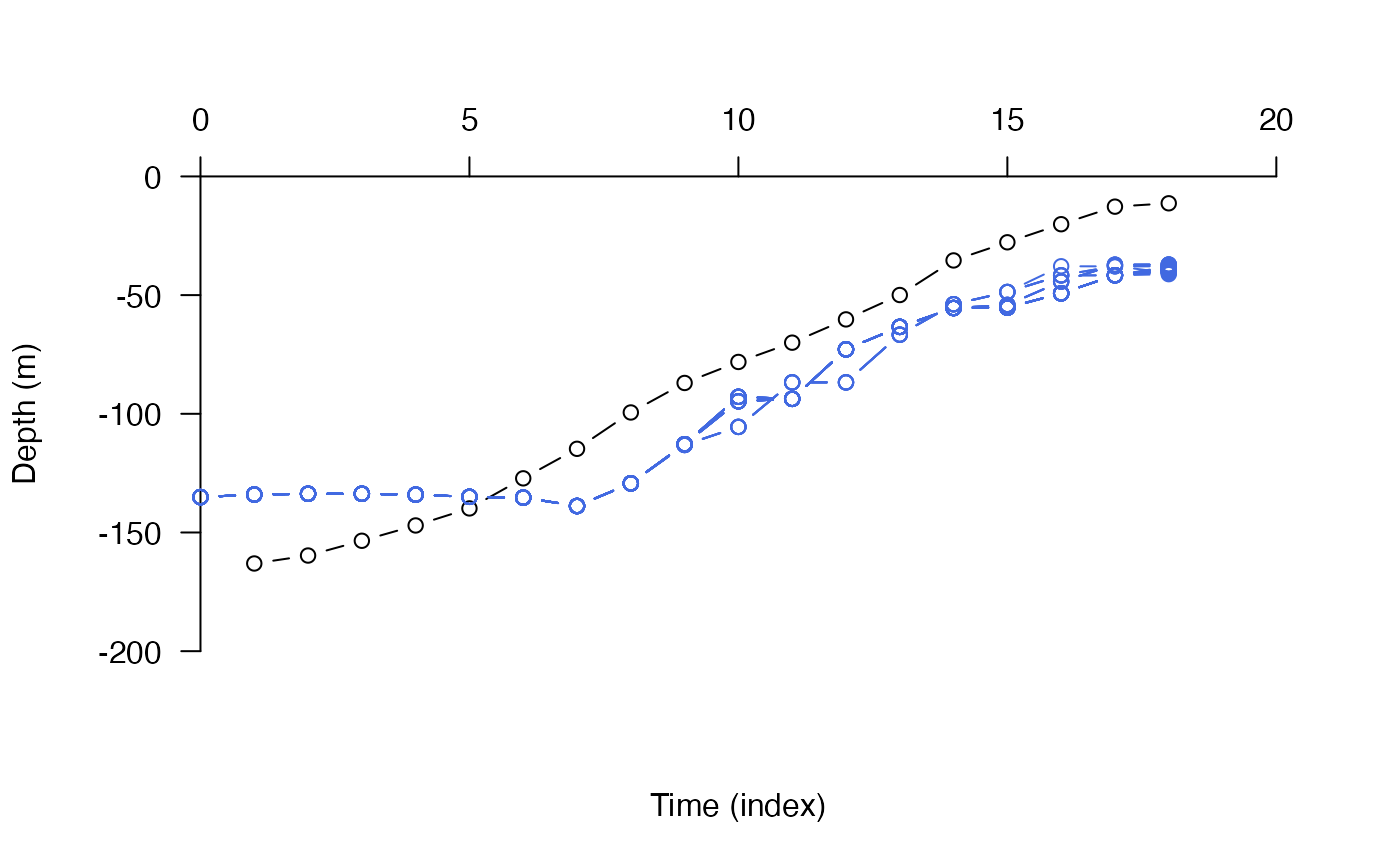
# There is a relatively large degree of mismatch here, which reflects
# ... the low resolution bathymetry data used for the algorithm.
pf_plot_1d(paths_1, dat_dc$args$archival)
 ## Examine paths
# Log likelihood
pf_loglik(paths_1)
#> path_id loglik delta
#> 1 4 -145.7709 0.00000000
#> 2 5 -145.8111 0.04017947
#> 3 3 -145.8431 0.07217439
#> 4 2 -145.9346 0.16376265
#> 5 1 -146.8934 1.12246741
#> 6 19 -147.6582 1.88729381
#> 7 24 -147.6644 1.89348096
#> 8 18 -147.6736 1.90275861
#> 9 23 -147.6798 1.90894575
#> 10 9 -147.6820 1.91112531
#> 11 14 -147.6882 1.91731246
#> 12 8 -147.6975 1.92659011
#> 13 13 -147.7037 1.93277725
#> 14 16 -147.7395 1.96864247
#> 15 17 -147.7395 1.96864247
#> 16 21 -147.7457 1.97482962
#> 17 22 -147.7457 1.97482962
#> 18 6 -147.7634 1.99247397
#> 19 7 -147.7634 1.99247397
#> 20 11 -147.7695 1.99866112
#> 21 12 -147.7695 1.99866112
#> 22 20 -151.9751 6.20417920
#> 23 25 -151.9813 6.21036635
#> 24 10 -151.9989 6.22801070
#> 25 15 -152.0051 6.23419785
# 2-d visualisation
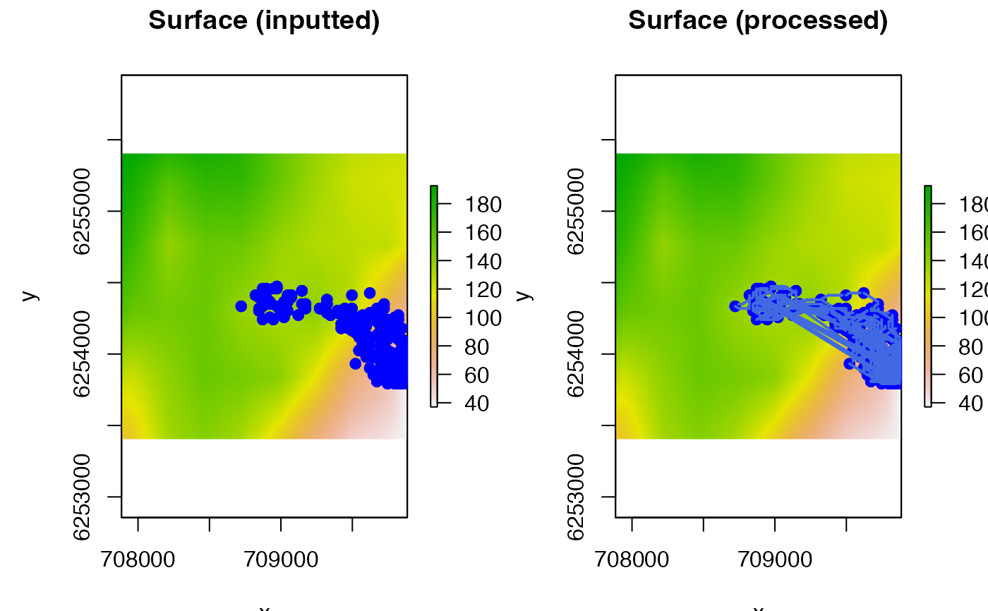
pf_plot_2d(paths_1, dat_dcpf_histories$args$bathy,
add_paths = list(length = 0.05)
)
#> prettyGraphics::pretty_map() CRS taken as: 'NA'.
#> Warning: zero-length arrow is of indeterminate angle and so skipped
#> Warning: zero-length arrow is of indeterminate angle and so skipped
#> Warning: zero-length arrow is of indeterminate angle and so skipped
#> Warning: zero-length arrow is of indeterminate angle and so skipped
#> Warning: zero-length arrow is of indeterminate angle and so skipped
#> Warning: zero-length arrow is of indeterminate angle and so skipped
#> Warning: zero-length arrow is of indeterminate angle and so skipped
## Examine paths
# Log likelihood
pf_loglik(paths_1)
#> path_id loglik delta
#> 1 4 -145.7709 0.00000000
#> 2 5 -145.8111 0.04017947
#> 3 3 -145.8431 0.07217439
#> 4 2 -145.9346 0.16376265
#> 5 1 -146.8934 1.12246741
#> 6 19 -147.6582 1.88729381
#> 7 24 -147.6644 1.89348096
#> 8 18 -147.6736 1.90275861
#> 9 23 -147.6798 1.90894575
#> 10 9 -147.6820 1.91112531
#> 11 14 -147.6882 1.91731246
#> 12 8 -147.6975 1.92659011
#> 13 13 -147.7037 1.93277725
#> 14 16 -147.7395 1.96864247
#> 15 17 -147.7395 1.96864247
#> 16 21 -147.7457 1.97482962
#> 17 22 -147.7457 1.97482962
#> 18 6 -147.7634 1.99247397
#> 19 7 -147.7634 1.99247397
#> 20 11 -147.7695 1.99866112
#> 21 12 -147.7695 1.99866112
#> 22 20 -151.9751 6.20417920
#> 23 25 -151.9813 6.21036635
#> 24 10 -151.9989 6.22801070
#> 25 15 -152.0051 6.23419785
# 2-d visualisation
pf_plot_2d(paths_1, dat_dcpf_histories$args$bathy,
add_paths = list(length = 0.05)
)
#> prettyGraphics::pretty_map() CRS taken as: 'NA'.
#> Warning: zero-length arrow is of indeterminate angle and so skipped
#> Warning: zero-length arrow is of indeterminate angle and so skipped
#> Warning: zero-length arrow is of indeterminate angle and so skipped
#> Warning: zero-length arrow is of indeterminate angle and so skipped
#> Warning: zero-length arrow is of indeterminate angle and so skipped
#> Warning: zero-length arrow is of indeterminate angle and so skipped
#> Warning: zero-length arrow is of indeterminate angle and so skipped
 # 3-d visualisation
pf_plot_3d(paths_1, dat_dcpf_histories$args$bathy)
#> Defining plot properties...
#> Producing plot...
#### Example (2): Re-calculate distances as shortest distances
## Implement flapper::pf()
# For this example, we need to increase the number of particles
# ... for Euclidean-based sampling to generate viable paths
# ... when we consider shortest distances
set.seed(1)
dcpf_args <- dat_dcpf_histories$args
dcpf_args$calc_distance_euclid_fast <- TRUE
dcpf_args$n <- 50
out_dcpf_2 <- do.call(pf, dcpf_args)
#> flapper::pf() called (@ 2023-08-29 15:45:48)...
#> ... Setting up function...
#> ... Determining the set of possible starting locations (t = 1)...
#> Warning: GEOS support is provided by the sf and terra packages among others
#> ... Implementing algorithm iteratively over time steps...
#> ... ... Time = 1...
#> ... ... ... Selecting candidate starting positions for the current time step...
#> ... ... ... For each particle, getting the possible positions for the next time step...
#> Warning: GEOS support is provided by the sf and terra packages among others
#> ... ... Time = 2...
#> ... ... ... Selecting candidate starting positions for the current time step...
#> ... ... ... For each particle, getting the possible positions for the next time step...
#> Warning: GEOS support is provided by the sf and terra packages among others
#> ... ... Time = 3...
#> ... ... ... Selecting candidate starting positions for the current time step...
#> ... ... ... For each particle, getting the possible positions for the next time step...
#> Warning: GEOS support is provided by the sf and terra packages among others
#> ... ... Time = 4...
#> ... ... ... Selecting candidate starting positions for the current time step...
#> ... ... ... For each particle, getting the possible positions for the next time step...
#> Warning: GEOS support is provided by the sf and terra packages among others
#> ... ... Time = 5...
#> ... ... ... Selecting candidate starting positions for the current time step...
#> ... ... ... For each particle, getting the possible positions for the next time step...
#> Warning: GEOS support is provided by the sf and terra packages among others
#> ... ... Time = 6...
#> ... ... ... Selecting candidate starting positions for the current time step...
#> ... ... ... For each particle, getting the possible positions for the next time step...
#> Warning: GEOS support is provided by the sf and terra packages among others
#> ... ... Time = 7...
#> ... ... ... Selecting candidate starting positions for the current time step...
#> ... ... ... For each particle, getting the possible positions for the next time step...
#> Warning: GEOS support is provided by the sf and terra packages among others
#> ... ... Time = 8...
#> ... ... ... Selecting candidate starting positions for the current time step...
#> ... ... ... For each particle, getting the possible positions for the next time step...
#> Warning: GEOS support is provided by the sf and terra packages among others
#> ... ... Time = 9...
#> ... ... ... Selecting candidate starting positions for the current time step...
#> ... ... ... For each particle, getting the possible positions for the next time step...
#> Warning: GEOS support is provided by the sf and terra packages among others
#> ... ... Time = 10...
#> ... ... ... Selecting candidate starting positions for the current time step...
#> ... ... ... For each particle, getting the possible positions for the next time step...
#> Warning: GEOS support is provided by the sf and terra packages among others
#> ... ... Time = 11...
#> ... ... ... Selecting candidate starting positions for the current time step...
#> ... ... ... For each particle, getting the possible positions for the next time step...
#> Warning: GEOS support is provided by the sf and terra packages among others
#> ... ... Time = 12...
#> ... ... ... Selecting candidate starting positions for the current time step...
#> ... ... ... For each particle, getting the possible positions for the next time step...
#> Warning: GEOS support is provided by the sf and terra packages among others
#> ... ... Time = 13...
#> ... ... ... Selecting candidate starting positions for the current time step...
#> ... ... ... For each particle, getting the possible positions for the next time step...
#> Warning: GEOS support is provided by the sf and terra packages among others
#> ... ... Time = 14...
#> ... ... ... Selecting candidate starting positions for the current time step...
#> ... ... ... For each particle, getting the possible positions for the next time step...
#> Warning: GEOS support is provided by the sf and terra packages among others
#> ... ... Time = 15...
#> ... ... ... Selecting candidate starting positions for the current time step...
#> ... ... ... For each particle, getting the possible positions for the next time step...
#> Warning: GEOS support is provided by the sf and terra packages among others
#> ... ... Time = 16...
#> ... ... ... Selecting candidate starting positions for the current time step...
#> ... ... ... For each particle, getting the possible positions for the next time step...
#> Warning: GEOS support is provided by the sf and terra packages among others
#> ... ... Time = 17...
#> ... ... ... Selecting candidate starting positions for the current time step...
#> ... ... ... For each particle, getting the possible positions for the next time step...
#> Warning: GEOS support is provided by the sf and terra packages among others
#> ... ... Time = 18...
#> ... ... ... Selecting candidate starting positions for the current time step...
#> ... flapper::pf() call completed (@ 2023-08-29 15:45:49) after ~0.01 minutes.
## Implement pf_simplify() using shortest distances
paths_2 <- pf_simplify(out_dcpf_2, calc_distance = "lcp")
#> flapper::pf_simplify() called (@ 2023-08-29 15:45:49)...
#> ... Getting pairwise cell movements based on calc_distance = 'lcp'...
#> ... Setting up LCP calculations...
#> ... ... Setting up cost-surface for calc_distance = 'lcp'...
#> flapper::lcp_costs() called (@ 2023-08-29 15:45:49)...
#> ... Defining transition matrices...
#> Warning: transition function gives negative values
#> ... Calculating distance matrices...
#> ... Assembling LCP costs...
#> ... flapper::lcp_costs() call completed (@ 2023-08-29 15:45:49) after ~0 minutes.
#> flapper::lcp_graph_surface() called (@ 2023-08-29 15:45:49)...
#> ... Defining nodes, edges and costs to make graph...
#> ... Constructing graph object...
#> ... flapper::lcp_graph_surface() call completed (@ 2023-08-29 15:45:49) after ~0 minutes.
#> ... ... Stepping through time steps to join coordinate pairs...
#> ... ... Identifying connected cells...
#> ... Assembling paths...
#> ... Formatting paths...
#> ... Adding cell coordinates and depths...
#> ... flapper::pf_simplify() call completed (@ 2023-08-29 15:45:50) after ~0.01 minutes.
# ... Duration: ~ 0.655 s
system.time(
invisible(utils::capture.output(
pf_simplify(out_dcpf_2, calc_distance = "lcp")
))
)
#> Warning: transition function gives negative values
#> user system elapsed
#> 0.490 0.039 0.636
## Demonstrate the LCP calculations are correct
paths_2_lcps <- lcp_interp(paths_2,
out_dcpf_2$args$bathy,
calc_distance = TRUE
)
#> flapper::lcp_interp() called (@ 2023-08-29 15:45:51)...
#> ... Setting up function...
#> ... Processing paths...
#> ... Calculating least-cost paths via flapper::lcp_over_surface()...
#> flapper::lcp_over_surface() called (@ 2023-08-29 15:45:51)...
#> ... Checking user inputs...
#> ... Defining cost matrix...
#> Warning: transition function gives negative values
# 3-d visualisation
pf_plot_3d(paths_1, dat_dcpf_histories$args$bathy)
#> Defining plot properties...
#> Producing plot...
#### Example (2): Re-calculate distances as shortest distances
## Implement flapper::pf()
# For this example, we need to increase the number of particles
# ... for Euclidean-based sampling to generate viable paths
# ... when we consider shortest distances
set.seed(1)
dcpf_args <- dat_dcpf_histories$args
dcpf_args$calc_distance_euclid_fast <- TRUE
dcpf_args$n <- 50
out_dcpf_2 <- do.call(pf, dcpf_args)
#> flapper::pf() called (@ 2023-08-29 15:45:48)...
#> ... Setting up function...
#> ... Determining the set of possible starting locations (t = 1)...
#> Warning: GEOS support is provided by the sf and terra packages among others
#> ... Implementing algorithm iteratively over time steps...
#> ... ... Time = 1...
#> ... ... ... Selecting candidate starting positions for the current time step...
#> ... ... ... For each particle, getting the possible positions for the next time step...
#> Warning: GEOS support is provided by the sf and terra packages among others
#> ... ... Time = 2...
#> ... ... ... Selecting candidate starting positions for the current time step...
#> ... ... ... For each particle, getting the possible positions for the next time step...
#> Warning: GEOS support is provided by the sf and terra packages among others
#> ... ... Time = 3...
#> ... ... ... Selecting candidate starting positions for the current time step...
#> ... ... ... For each particle, getting the possible positions for the next time step...
#> Warning: GEOS support is provided by the sf and terra packages among others
#> ... ... Time = 4...
#> ... ... ... Selecting candidate starting positions for the current time step...
#> ... ... ... For each particle, getting the possible positions for the next time step...
#> Warning: GEOS support is provided by the sf and terra packages among others
#> ... ... Time = 5...
#> ... ... ... Selecting candidate starting positions for the current time step...
#> ... ... ... For each particle, getting the possible positions for the next time step...
#> Warning: GEOS support is provided by the sf and terra packages among others
#> ... ... Time = 6...
#> ... ... ... Selecting candidate starting positions for the current time step...
#> ... ... ... For each particle, getting the possible positions for the next time step...
#> Warning: GEOS support is provided by the sf and terra packages among others
#> ... ... Time = 7...
#> ... ... ... Selecting candidate starting positions for the current time step...
#> ... ... ... For each particle, getting the possible positions for the next time step...
#> Warning: GEOS support is provided by the sf and terra packages among others
#> ... ... Time = 8...
#> ... ... ... Selecting candidate starting positions for the current time step...
#> ... ... ... For each particle, getting the possible positions for the next time step...
#> Warning: GEOS support is provided by the sf and terra packages among others
#> ... ... Time = 9...
#> ... ... ... Selecting candidate starting positions for the current time step...
#> ... ... ... For each particle, getting the possible positions for the next time step...
#> Warning: GEOS support is provided by the sf and terra packages among others
#> ... ... Time = 10...
#> ... ... ... Selecting candidate starting positions for the current time step...
#> ... ... ... For each particle, getting the possible positions for the next time step...
#> Warning: GEOS support is provided by the sf and terra packages among others
#> ... ... Time = 11...
#> ... ... ... Selecting candidate starting positions for the current time step...
#> ... ... ... For each particle, getting the possible positions for the next time step...
#> Warning: GEOS support is provided by the sf and terra packages among others
#> ... ... Time = 12...
#> ... ... ... Selecting candidate starting positions for the current time step...
#> ... ... ... For each particle, getting the possible positions for the next time step...
#> Warning: GEOS support is provided by the sf and terra packages among others
#> ... ... Time = 13...
#> ... ... ... Selecting candidate starting positions for the current time step...
#> ... ... ... For each particle, getting the possible positions for the next time step...
#> Warning: GEOS support is provided by the sf and terra packages among others
#> ... ... Time = 14...
#> ... ... ... Selecting candidate starting positions for the current time step...
#> ... ... ... For each particle, getting the possible positions for the next time step...
#> Warning: GEOS support is provided by the sf and terra packages among others
#> ... ... Time = 15...
#> ... ... ... Selecting candidate starting positions for the current time step...
#> ... ... ... For each particle, getting the possible positions for the next time step...
#> Warning: GEOS support is provided by the sf and terra packages among others
#> ... ... Time = 16...
#> ... ... ... Selecting candidate starting positions for the current time step...
#> ... ... ... For each particle, getting the possible positions for the next time step...
#> Warning: GEOS support is provided by the sf and terra packages among others
#> ... ... Time = 17...
#> ... ... ... Selecting candidate starting positions for the current time step...
#> ... ... ... For each particle, getting the possible positions for the next time step...
#> Warning: GEOS support is provided by the sf and terra packages among others
#> ... ... Time = 18...
#> ... ... ... Selecting candidate starting positions for the current time step...
#> ... flapper::pf() call completed (@ 2023-08-29 15:45:49) after ~0.01 minutes.
## Implement pf_simplify() using shortest distances
paths_2 <- pf_simplify(out_dcpf_2, calc_distance = "lcp")
#> flapper::pf_simplify() called (@ 2023-08-29 15:45:49)...
#> ... Getting pairwise cell movements based on calc_distance = 'lcp'...
#> ... Setting up LCP calculations...
#> ... ... Setting up cost-surface for calc_distance = 'lcp'...
#> flapper::lcp_costs() called (@ 2023-08-29 15:45:49)...
#> ... Defining transition matrices...
#> Warning: transition function gives negative values
#> ... Calculating distance matrices...
#> ... Assembling LCP costs...
#> ... flapper::lcp_costs() call completed (@ 2023-08-29 15:45:49) after ~0 minutes.
#> flapper::lcp_graph_surface() called (@ 2023-08-29 15:45:49)...
#> ... Defining nodes, edges and costs to make graph...
#> ... Constructing graph object...
#> ... flapper::lcp_graph_surface() call completed (@ 2023-08-29 15:45:49) after ~0 minutes.
#> ... ... Stepping through time steps to join coordinate pairs...
#> ... ... Identifying connected cells...
#> ... Assembling paths...
#> ... Formatting paths...
#> ... Adding cell coordinates and depths...
#> ... flapper::pf_simplify() call completed (@ 2023-08-29 15:45:50) after ~0.01 minutes.
# ... Duration: ~ 0.655 s
system.time(
invisible(utils::capture.output(
pf_simplify(out_dcpf_2, calc_distance = "lcp")
))
)
#> Warning: transition function gives negative values
#> user system elapsed
#> 0.490 0.039 0.636
## Demonstrate the LCP calculations are correct
paths_2_lcps <- lcp_interp(paths_2,
out_dcpf_2$args$bathy,
calc_distance = TRUE
)
#> flapper::lcp_interp() called (@ 2023-08-29 15:45:51)...
#> ... Setting up function...
#> ... Processing paths...
#> ... Calculating least-cost paths via flapper::lcp_over_surface()...
#> flapper::lcp_over_surface() called (@ 2023-08-29 15:45:51)...
#> ... Checking user inputs...
#> ... Defining cost matrix...
#> Warning: transition function gives negative values
 #> ... Using method = 'cppRouting'...
#> ... ... Defining nodes, edges and costs to make graph...
#> ... ... Constructing graph object...
#> ... ... Implementing bi algorithm to compute least-cost paths(s)...
#> ... flapper::lcp_over_surface() call completed (@ 2023-08-29 15:45:52) after ~0.01 minutes.
#> ... Summarising distances for each least-cost path...
#> ... flapper::lcp_interp() call completed (@ 2023-08-29 15:45:52) after ~0.01 minutes.
head(cbind(paths_2$dist, paths_2_lcps$dist_lcp$dist))
#> [,1] [,2]
#> [1,] NA NA
#> [2,] 60.38712 NA
#> [3,] 60.38712 NA
#> [4,] 60.37633 NA
#> [5,] 156.07347 NA
#> [6,] 135.35917 NA
## Trial options for increasing speed of shortest-distance calculations
# Speed up shortest-distance calculations via (a) the graph:
# ... Duration: ~0.495 s
# ... Note that you may achieve further speed improvements via
# ... a simplified/contracted graph
# ... ... see cppRouting::cpp_simplify()
# ... ... see cppRouting::cpp_contract()
costs <- lcp_costs(out_dcpf_2$args$bathy)
#> flapper::lcp_costs() called (@ 2023-08-29 15:45:52)...
#> ... Defining transition matrices...
#> Warning: transition function gives negative values
#> ... Calculating distance matrices...
#> ... Assembling LCP costs...
#> ... flapper::lcp_costs() call completed (@ 2023-08-29 15:45:52) after ~0 minutes.
graph <- lcp_graph_surface(out_dcpf_2$args$bathy, costs$dist_total)
#> flapper::lcp_graph_surface() called (@ 2023-08-29 15:45:52)...
#> ... Defining nodes, edges and costs to make graph...
#> ... Constructing graph object...
#> ... flapper::lcp_graph_surface() call completed (@ 2023-08-29 15:45:52) after ~0 minutes.
system.time(
invisible(utils::capture.output(
pf_simplify(out_dcpf_2,
calc_distance = "lcp",
calc_distance_graph = graph
)
))
)
#> user system elapsed
#> 0.329 0.023 0.296
# Speed up shortest-distance calculations via (b) the lower Euclid dist limit
# ... Duration: ~0.493 s
costs <- lcp_costs(out_dcpf_2$args$bathy)
#> flapper::lcp_costs() called (@ 2023-08-29 15:45:53)...
#> ... Defining transition matrices...
#> Warning: transition function gives negative values
#> ... Calculating distance matrices...
#> ... Assembling LCP costs...
#> ... flapper::lcp_costs() call completed (@ 2023-08-29 15:45:53) after ~0 minutes.
graph <- lcp_graph_surface(out_dcpf_2$args$bathy, costs$dist_total)
#> flapper::lcp_graph_surface() called (@ 2023-08-29 15:45:53)...
#> ... Defining nodes, edges and costs to make graph...
#> ... Constructing graph object...
#> ... flapper::lcp_graph_surface() call completed (@ 2023-08-29 15:45:53) after ~0 minutes.
system.time(
invisible(utils::capture.output(
pf_simplify(out_dcpf_2,
calc_distance = "lcp",
calc_distance_graph = graph,
calc_distance_limit = 100
)
))
)
#> user system elapsed
#> 0.308 0.020 0.268
# Speed up shortest-distance calculations via (c) the barrier
# ... Duration: ~1.411 s (much slower in this example)
coastline <- sf::st_as_sf(dat_coast)
sf::st_crs(coastline) <- NA
system.time(
invisible(utils::capture.output(
pf_simplify(out_dcpf_2,
calc_distance = "lcp",
calc_distance_graph = graph,
calc_distance_limit = 100,
calc_distance_barrier = coastline
)
))
)
#> Warning: The CRSs of 'bathy' and 'calc_distance_barrier' are not identical.
#> -- details: Modes: S4, characterAttributes: < Modes: list, NULL >Attributes: < Lengths: 2, 0 >Attributes: < names for target but not for current >Attributes: < current is not list-like >.
#> -- bathy CRS: 'NA'.
#> -- calc_distance_barrier CRS: ''.
#> user system elapsed
#> 0.409 0.033 0.390
# Speed up calculations via (d) mobility limits
# ... (In the examples above, the mobility parameters
# ... can be extracted from out_dcpf_2,
# ... so specifying them directly here in this example makes
# ... no material difference, but this is not necessarily the case
# ... if pf() has been implemented without mobility parameters).
system.time(
invisible(utils::capture.output(
pf_simplify(out_dcpf_2,
calc_distance = "lcp",
calc_distance_graph = graph,
calc_distance_limit = 100,
mobility = 200,
mobility_from_origin = 200
)
))
)
#> user system elapsed
#> 0.308 0.027 0.395
# Speed up calculations via (e) parallelisation
# ... see the details in the documentation.
#### Example (3): Restrict the number of routes to each cell at each time step
# Implement approach for different numbers of copies
# Since we only have sampled a small number of particles for this simulation
# ... this does not make any difference here, but it can dramatically reduce
# ... the time taken to assemble paths and prevent vector memory issues.
paths_3a <- pf_simplify(dat_dcpf_histories, max_n_copies = 1)
#> flapper::pf_simplify() called (@ 2023-08-29 15:45:55)...
#> ... Getting pairwise cell movements based on calc_distance = 'euclid'...
#> ... ... Stepping through time steps to join coordinate pairs...
#> ... ... Identifying connected cells...
#> ... Assembling paths...
#> ... Formatting paths...
#> ... Adding cell coordinates and depths...
#> ... flapper::pf_simplify() call completed (@ 2023-08-29 15:45:55) after ~0 minutes.
paths_3b <- pf_simplify(dat_dcpf_histories, max_n_copies = 5)
#> flapper::pf_simplify() called (@ 2023-08-29 15:45:55)...
#> ... Getting pairwise cell movements based on calc_distance = 'euclid'...
#> ... ... Stepping through time steps to join coordinate pairs...
#> ... ... Identifying connected cells...
#> ... Assembling paths...
#> ... Formatting paths...
#> ... Adding cell coordinates and depths...
#> ... flapper::pf_simplify() call completed (@ 2023-08-29 15:45:55) after ~0 minutes.
paths_3c <- pf_simplify(dat_dcpf_histories, max_n_copies = 7)
#> flapper::pf_simplify() called (@ 2023-08-29 15:45:55)...
#> ... Getting pairwise cell movements based on calc_distance = 'euclid'...
#> ... ... Stepping through time steps to join coordinate pairs...
#> ... ... Identifying connected cells...
#> ... Assembling paths...
#> ... Formatting paths...
#> ... Adding cell coordinates and depths...
#> ... flapper::pf_simplify() call completed (@ 2023-08-29 15:45:56) after ~0 minutes.
# Compare the number of paths retained
unique(paths_3a$path_id)
#> [1] 1 2 3 4 5 6 7 8 9 10
unique(paths_3b$path_id)
#> [1] 1 2 3 4 5 6 7 8 9 10 11 12 13 14 15 16 17 18 19 20 21 22 23 24 25
#> [26] 26 27 28 29 30 31 32 33 34 35 36 37 38 39 40 41 42 43 44 45 46 47 48 49 50
unique(paths_3c$path_id)
#> [1] 1 2 3 4 5 6 7 8 9 10 11 12 13 14 15 16 17 18 19 20 21 22 23 24 25
#> [26] 26 27 28 29 30 31 32 33 34 35 36 37 38 39 40 41 42 43 44 45 46 47 48 49 50
#> [51] 51 52 53 54 55 56 57 58 59 60 61 62 63 64 65 66 67 68 69 70
#### Example (4): Change the sampling method used to retain paths
# Again, this doesn't make a difference here, but it can when there are
# ... more particles.
paths_4a <- pf_simplify(dat_dcpf_histories,
max_n_copies = 5,
max_n_copies_sampler = "random"
)
#> flapper::pf_simplify() called (@ 2023-08-29 15:45:56)...
#> ... Getting pairwise cell movements based on calc_distance = 'euclid'...
#> ... ... Stepping through time steps to join coordinate pairs...
#> ... ... Identifying connected cells...
#> ... Assembling paths...
#> ... Formatting paths...
#> ... Adding cell coordinates and depths...
#> ... flapper::pf_simplify() call completed (@ 2023-08-29 15:45:56) after ~0 minutes.
paths_4b <- pf_simplify(dat_dcpf_histories,
max_n_copies = 5,
max_n_copies_sampler = "weighted"
)
#> flapper::pf_simplify() called (@ 2023-08-29 15:45:56)...
#> ... Getting pairwise cell movements based on calc_distance = 'euclid'...
#> ... ... Stepping through time steps to join coordinate pairs...
#> ... ... Identifying connected cells...
#> ... Assembling paths...
#> ... Formatting paths...
#> ... Adding cell coordinates and depths...
#> ... flapper::pf_simplify() call completed (@ 2023-08-29 15:45:56) after ~0 minutes.
paths_4c <- pf_simplify(dat_dcpf_histories,
max_n_copies = 5,
max_n_copies_sampler = "max"
)
#> flapper::pf_simplify() called (@ 2023-08-29 15:45:56)...
#> ... Getting pairwise cell movements based on calc_distance = 'euclid'...
#> ... ... Stepping through time steps to join coordinate pairs...
#> ... ... Identifying connected cells...
#> ... Assembling paths...
#> ... Formatting paths...
#> ... Adding cell coordinates and depths...
#> ... flapper::pf_simplify() call completed (@ 2023-08-29 15:45:57) after ~0.01 minutes.
# Compare retained paths
pf_loglik(paths_3a)
#> path_id loglik delta
#> 1 1 -145.7709 0.00000000
#> 2 3 -145.8111 0.04017947
#> 3 4 -145.8431 0.07217439
#> 4 5 -145.9346 0.16376265
#> 5 2 -146.8934 1.12246741
#> 6 7 -147.6820 1.91112531
#> 7 8 -147.6975 1.92659011
#> 8 6 -147.7634 1.99247397
#> 9 9 -147.7634 1.99247397
#> 10 10 -151.9989 6.22801070
pf_loglik(paths_3b)
#> path_id loglik delta
#> 1 1 -145.7709 0.00000000
#> 2 2 -145.7709 0.00000000
#> 3 3 -145.7709 0.00000000
#> 4 4 -145.7709 0.00000000
#> 5 5 -145.7709 0.00000000
#> 6 11 -145.8111 0.04017947
#> 7 12 -145.8111 0.04017947
#> 8 13 -145.8111 0.04017947
#> 9 14 -145.8111 0.04017947
#> 10 15 -145.8111 0.04017947
#> 11 16 -145.8431 0.07217439
#> 12 17 -145.8431 0.07217439
#> 13 18 -145.8431 0.07217439
#> 14 19 -145.8431 0.07217439
#> 15 20 -145.8431 0.07217439
#> 16 21 -145.9346 0.16376265
#> 17 22 -145.9346 0.16376265
#> 18 23 -145.9346 0.16376265
#> 19 24 -145.9346 0.16376265
#> 20 25 -145.9346 0.16376265
#> 21 6 -146.8934 1.12246741
#> 22 7 -146.8934 1.12246741
#> 23 8 -146.8934 1.12246741
#> 24 9 -146.8934 1.12246741
#> 25 10 -146.8934 1.12246741
#> 26 31 -147.6582 1.88729381
#> 27 34 -147.6582 1.88729381
#> 28 37 -147.6736 1.90275861
#> 29 38 -147.6736 1.90275861
#> 30 39 -147.6736 1.90275861
#> 31 40 -147.6736 1.90275861
#> 32 32 -147.6882 1.91731246
#> 33 33 -147.6882 1.91731246
#> 34 35 -147.6882 1.91731246
#> 35 36 -147.7037 1.93277725
#> 36 27 -147.7395 1.96864247
#> 37 28 -147.7395 1.96864247
#> 38 42 -147.7395 1.96864247
#> 39 43 -147.7395 1.96864247
#> 40 26 -147.7695 1.99866112
#> 41 29 -147.7695 1.99866112
#> 42 30 -147.7695 1.99866112
#> 43 41 -147.7695 1.99866112
#> 44 44 -147.7695 1.99866112
#> 45 45 -147.7695 1.99866112
#> 46 46 -151.9751 6.20417920
#> 47 47 -151.9751 6.20417920
#> 48 49 -151.9751 6.20417920
#> 49 48 -152.0051 6.23419785
#> 50 50 -152.0051 6.23419785
pf_loglik(paths_3c)
#> path_id loglik delta
#> 1 1 -145.7709 0.00000000
#> 2 2 -145.7709 0.00000000
#> 3 3 -145.7709 0.00000000
#> 4 4 -145.7709 0.00000000
#> 5 5 -145.7709 0.00000000
#> 6 6 -145.7709 0.00000000
#> 7 7 -145.7709 0.00000000
#> 8 15 -145.8111 0.04017947
#> 9 16 -145.8111 0.04017947
#> 10 17 -145.8111 0.04017947
#> 11 18 -145.8111 0.04017947
#> 12 19 -145.8111 0.04017947
#> 13 20 -145.8111 0.04017947
#> 14 21 -145.8111 0.04017947
#> 15 22 -145.8431 0.07217439
#> 16 23 -145.8431 0.07217439
#> 17 24 -145.8431 0.07217439
#> 18 25 -145.8431 0.07217439
#> 19 26 -145.8431 0.07217439
#> 20 27 -145.8431 0.07217439
#> 21 28 -145.8431 0.07217439
#> 22 29 -145.9346 0.16376265
#> 23 30 -145.9346 0.16376265
#> 24 31 -145.9346 0.16376265
#> 25 32 -145.9346 0.16376265
#> 26 33 -145.9346 0.16376265
#> 27 34 -145.9346 0.16376265
#> 28 35 -145.9346 0.16376265
#> 29 8 -146.8934 1.12246741
#> 30 9 -146.8934 1.12246741
#> 31 10 -146.8934 1.12246741
#> 32 11 -146.8934 1.12246741
#> 33 12 -146.8934 1.12246741
#> 34 13 -146.8934 1.12246741
#> 35 14 -146.8934 1.12246741
#> 36 43 -147.6644 1.89348096
#> 37 44 -147.6644 1.89348096
#> 38 45 -147.6644 1.89348096
#> 39 47 -147.6644 1.89348096
#> 40 48 -147.6644 1.89348096
#> 41 49 -147.6644 1.89348096
#> 42 51 -147.6798 1.90894575
#> 43 55 -147.6798 1.90894575
#> 44 56 -147.6798 1.90894575
#> 45 46 -147.6820 1.91112531
#> 46 50 -147.6975 1.92659011
#> 47 52 -147.6975 1.92659011
#> 48 53 -147.6975 1.92659011
#> 49 54 -147.6975 1.92659011
#> 50 36 -147.7457 1.97482962
#> 51 38 -147.7457 1.97482962
#> 52 39 -147.7457 1.97482962
#> 53 42 -147.7457 1.97482962
#> 54 58 -147.7457 1.97482962
#> 55 60 -147.7457 1.97482962
#> 56 62 -147.7457 1.97482962
#> 57 63 -147.7457 1.97482962
#> 58 37 -147.7634 1.99247397
#> 59 40 -147.7634 1.99247397
#> 60 41 -147.7634 1.99247397
#> 61 57 -147.7634 1.99247397
#> 62 59 -147.7634 1.99247397
#> 63 61 -147.7634 1.99247397
#> 64 64 -151.9813 6.21036635
#> 65 66 -151.9813 6.21036635
#> 66 67 -151.9813 6.21036635
#> 67 69 -151.9813 6.21036635
#> 68 70 -151.9813 6.21036635
#> 69 65 -151.9989 6.22801070
#> 70 68 -151.9989 6.22801070
#### Example (5): Set the maximum number of paths for reconstruction (for speed)
# Reconstruct all paths (note you may experience vector memory limitations)
# unique(pf_simplify(dat_dcpf_histories, max_n_paths = NULL)$path_id)
# Reconstruct one path
unique(pf_simplify(dat_dcpf_histories, max_n_paths = 1)$path_id)
#> flapper::pf_simplify() called (@ 2023-08-29 15:45:57)...
#> ... Getting pairwise cell movements based on calc_distance = 'euclid'...
#> ... ... Stepping through time steps to join coordinate pairs...
#> ... ... Identifying connected cells...
#> ... Assembling paths...
#> ... Formatting paths...
#> ... Adding cell coordinates and depths...
#> ... flapper::pf_simplify() call completed (@ 2023-08-29 15:45:57) after ~0 minutes.
#> [1] 1
# Reconstruct (at most) five paths
unique(pf_simplify(dat_dcpf_histories, max_n_paths = 5)$path_id)
#> flapper::pf_simplify() called (@ 2023-08-29 15:45:57)...
#> ... Getting pairwise cell movements based on calc_distance = 'euclid'...
#> ... ... Stepping through time steps to join coordinate pairs...
#> ... ... Identifying connected cells...
#> ... Assembling paths...
#> ... Formatting paths...
#> ... Adding cell coordinates and depths...
#> ... flapper::pf_simplify() call completed (@ 2023-08-29 15:45:57) after ~0 minutes.
#> [1] 1 2 3 4 5
#### Example (6): Retain/drop the origin, if specified
# For the example particle histories, an origin was specified
dat_dcpf_histories$args$origin
#> [,1] [,2]
#> [1,] 708886.3 6254404
# This is included as 'timestep = 0' in the returned dataframe
# ... with the coordinates re-defined on bathy:
paths_5a <- pf_simplify(dat_dcpf_histories)
#> flapper::pf_simplify() called (@ 2023-08-29 15:45:57)...
#> ... Getting pairwise cell movements based on calc_distance = 'euclid'...
#> ... ... Stepping through time steps to join coordinate pairs...
#> ... ... Identifying connected cells...
#> ... Assembling paths...
#> ... Formatting paths...
#> ... Adding cell coordinates and depths...
#> ... flapper::pf_simplify() call completed (@ 2023-08-29 15:45:57) after ~0 minutes.
paths_5a[1, c("cell_x", "cell_y")]
#> cell_x cell_y
#> 1 708897.1 6254392
raster::xyFromCell(
dat_dcpf_histories$args$bathy,
raster::cellFromXY(
dat_dcpf_histories$args$bathy,
dat_dcpf_histories$args$origin
)
)
#> x y
#> [1,] 708897.1 6254392
head(paths_5a)
#> path_id timestep cell_id cell_x cell_y cell_z cell_pr dist
#> 1 1 0 3241 708897.1 6254392 135.0958 1.000000e+00 NA
#> 2 1 1 3722 708922.1 6254242 134.0199 1.808832e-05 152.06906
#> 3 1 2 3243 708947.1 6254392 133.6996 1.663445e-05 152.06906
#> 4 1 3 3166 709022.1 6254416 133.6938 1.569277e-04 79.05694
#> 5 1 4 3006 709022.1 6254466 134.0630 1.826367e-04 50.00000
#> 6 1 5 3009 709097.1 6254466 134.9762 1.547789e-04 75.00000
# If specified, the origin is dropped with add_origin = FALSE
paths_5b <- pf_simplify(dat_dcpf_histories, add_origin = FALSE)
#> flapper::pf_simplify() called (@ 2023-08-29 15:45:57)...
#> ... Getting pairwise cell movements based on calc_distance = 'euclid'...
#> ... ... Stepping through time steps to join coordinate pairs...
#> ... ... Identifying connected cells...
#> ... Assembling paths...
#> ... Formatting paths...
#> ... Adding cell coordinates and depths...
#> ... flapper::pf_simplify() call completed (@ 2023-08-29 15:45:57) after ~0 minutes.
head(paths_5b)
#> path_id timestep cell_id cell_x cell_y cell_z cell_pr dist
#> 1 1 1 3722 708922.1 6254242 134.0199 1.808832e-05 152.06906
#> 2 1 2 3243 708947.1 6254392 133.6996 1.663445e-05 152.06906
#> 3 1 3 3166 709022.1 6254416 133.6938 1.569277e-04 79.05694
#> 4 1 4 3006 709022.1 6254466 134.0630 1.826367e-04 50.00000
#> 5 1 5 3009 709097.1 6254466 134.9762 1.547789e-04 75.00000
#> 6 1 6 3329 709097.1 6254366 135.3115 1.049538e-04 100.00000
#### Example (6) Get particle samples for connected particles
## Implement DCPF with more particles for demonstration purposes
set.seed(1)
dcpf_args <- dat_dcpf_histories$args
dcpf_args$calc_distance_euclid_fast <- TRUE
dcpf_args$n <- 250
out_dcpf_6a <- do.call(pf, dcpf_args)
#> flapper::pf() called (@ 2023-08-29 15:45:57)...
#> ... Setting up function...
#> ... Determining the set of possible starting locations (t = 1)...
#> Warning: GEOS support is provided by the sf and terra packages among others
#> ... Implementing algorithm iteratively over time steps...
#> ... ... Time = 1...
#> ... ... ... Selecting candidate starting positions for the current time step...
#> ... ... ... For each particle, getting the possible positions for the next time step...
#> Warning: GEOS support is provided by the sf and terra packages among others
#> ... ... Time = 2...
#> ... ... ... Selecting candidate starting positions for the current time step...
#> ... ... ... For each particle, getting the possible positions for the next time step...
#> Warning: GEOS support is provided by the sf and terra packages among others
#> ... ... Time = 3...
#> ... ... ... Selecting candidate starting positions for the current time step...
#> ... ... ... For each particle, getting the possible positions for the next time step...
#> Warning: GEOS support is provided by the sf and terra packages among others
#> ... ... Time = 4...
#> ... ... ... Selecting candidate starting positions for the current time step...
#> ... ... ... For each particle, getting the possible positions for the next time step...
#> Warning: GEOS support is provided by the sf and terra packages among others
#> ... ... Time = 5...
#> ... ... ... Selecting candidate starting positions for the current time step...
#> ... ... ... For each particle, getting the possible positions for the next time step...
#> Warning: GEOS support is provided by the sf and terra packages among others
#> ... ... Time = 6...
#> ... ... ... Selecting candidate starting positions for the current time step...
#> ... ... ... For each particle, getting the possible positions for the next time step...
#> Warning: GEOS support is provided by the sf and terra packages among others
#> ... ... Time = 7...
#> ... ... ... Selecting candidate starting positions for the current time step...
#> ... ... ... For each particle, getting the possible positions for the next time step...
#> Warning: GEOS support is provided by the sf and terra packages among others
#> ... ... Time = 8...
#> ... ... ... Selecting candidate starting positions for the current time step...
#> ... ... ... For each particle, getting the possible positions for the next time step...
#> Warning: GEOS support is provided by the sf and terra packages among others
#> ... ... Time = 9...
#> ... ... ... Selecting candidate starting positions for the current time step...
#> ... ... ... For each particle, getting the possible positions for the next time step...
#> Warning: GEOS support is provided by the sf and terra packages among others
#> ... ... Time = 10...
#> ... ... ... Selecting candidate starting positions for the current time step...
#> ... ... ... For each particle, getting the possible positions for the next time step...
#> Warning: GEOS support is provided by the sf and terra packages among others
#> ... ... Time = 11...
#> ... ... ... Selecting candidate starting positions for the current time step...
#> ... ... ... For each particle, getting the possible positions for the next time step...
#> Warning: GEOS support is provided by the sf and terra packages among others
#> ... ... Time = 12...
#> ... ... ... Selecting candidate starting positions for the current time step...
#> ... ... ... For each particle, getting the possible positions for the next time step...
#> Warning: GEOS support is provided by the sf and terra packages among others
#> ... ... Time = 13...
#> ... ... ... Selecting candidate starting positions for the current time step...
#> ... ... ... For each particle, getting the possible positions for the next time step...
#> Warning: GEOS support is provided by the sf and terra packages among others
#> ... ... Time = 14...
#> ... ... ... Selecting candidate starting positions for the current time step...
#> ... ... ... For each particle, getting the possible positions for the next time step...
#> Warning: GEOS support is provided by the sf and terra packages among others
#> ... ... Time = 15...
#> ... ... ... Selecting candidate starting positions for the current time step...
#> ... ... ... For each particle, getting the possible positions for the next time step...
#> Warning: GEOS support is provided by the sf and terra packages among others
#> ... ... Time = 16...
#> ... ... ... Selecting candidate starting positions for the current time step...
#> ... ... ... For each particle, getting the possible positions for the next time step...
#> Warning: GEOS support is provided by the sf and terra packages among others
#> ... ... Time = 17...
#> ... ... ... Selecting candidate starting positions for the current time step...
#> ... ... ... For each particle, getting the possible positions for the next time step...
#> Warning: GEOS support is provided by the sf and terra packages among others
#> ... ... Time = 18...
#> ... ... ... Selecting candidate starting positions for the current time step...
#> ... flapper::pf() call completed (@ 2023-08-29 15:46:01) after ~0.06 minutes.
head(out_dcpf_6a$history[[1]])
#> id_current pr_current timestep
#> 1 3243 2.425569e-04 1
#> 2 2921 1.312336e-04 1
#> 3 3396 3.947544e-05 1
#> 4 3159 2.364016e-04 1
#> 5 3320 2.525012e-04 1
#> 6 3237 1.312336e-04 1
## Extract particle samples for connected particles
# There may be multiple records of any given cell at any given time step
# ... due to sampling with replacement.
out_dcpf_6b <- pf_simplify(out_dcpf_6a, return = "archive")
#> flapper::pf_simplify() called (@ 2023-08-29 15:46:01)...
#> ... Getting pairwise cell movements based on calc_distance = 'euclid'...
#> ... ... Stepping through time steps to join coordinate pairs...
#> ... ... Identifying connected cells...
#> ... ... Processing connected cells for return = 'archive'...
#> ... flapper::pf_simplify() call completed (@ 2023-08-29 15:46:01) after ~0 minutes.
head(out_dcpf_6b$history[[1]])
#> timestep id_previous id_current dist_current pr_current
#> 1 1 3241 2838 145.7738 2.416378e-05
#> 2 1 3241 2839 134.6291 3.947544e-05
#> 3 1 3241 2841 125.0000 5.845148e-05
#> 4 1 3241 2842 127.4755 5.302119e-05
#> 5 1 3241 2917 141.4214 2.938080e-05
#> 6 1 3241 2918 125.0000 5.845148e-05
table(duplicated(out_dcpf_6b$history[[1]]$id_current))
#>
#> FALSE
#> 90
## Extract particle samples for connected particles,
# ... with only the most likely record of each particle returned.
# We can implement the approach using out_dcpf_6b
# ... to skip distance calculations.
# Now, there is only one (the most likely) record of sampled cells
# ... at each time step.
out_dcpf_6c <- pf_simplify(out_dcpf_6b,
summarise_pr = TRUE,
return = "archive"
)
#> flapper::pf_simplify() called (@ 2023-08-29 15:46:01)...
#> ... ... Processing connected cells for return = 'archive'...
#> ... flapper::pf_simplify() call completed (@ 2023-08-29 15:46:01) after ~0.01 minutes.
head(out_dcpf_6c$history[[1]])
#> timestep id_previous id_current dist_current pr_current
#> 1 1 3241 2838 145.7738 0.002078627
#> 2 1 3241 2839 134.6291 0.003395774
#> 3 1 3241 2841 125.0000 0.005028139
#> 4 1 3241 2842 127.4755 0.004561012
#> 5 1 3241 2917 141.4214 0.002527408
#> 6 1 3241 2918 125.0000 0.005028139
table(duplicated(out_dcpf_6c$history[[1]]$id_current))
#>
#> FALSE
#> 90
## Make movement paths
# Again, we use out_dcpf_6b to skip distance calculations.
out_dcpf_6d <- pf_simplify(out_dcpf_6b,
max_n_copies = 2L,
return = "path"
)
#> flapper::pf_simplify() called (@ 2023-08-29 15:46:01)...
#> ... Assembling paths...
#> ... Formatting paths...
#> ... Adding cell coordinates and depths...
#> ... flapper::pf_simplify() call completed (@ 2023-08-29 15:46:05) after ~0.07 minutes.
## Compare resultant maps
# The map for all particles is influenced by particles that were 'dead ends',
# ... which isn't ideal for a map of space use.
# The map for connected samples deals with this problem, but is influenced by
# ... the total number of samples of each cell, rather than the number of time steps
# ... in which the individual could have been located in a given cell.
# The map for unique, connected samples deals with this issue, so that scores
# ... represent the number of time steps in which the individual could have occupied
# ... a given cell, over the length of the time series.
# The map for the paths are sparser because paths have only been reconstructed
# ... for a sample of sampled particles.
pp <- par(mfrow = c(2, 2), oma = c(2, 2, 2, 2), mar = c(2, 4, 2, 4))
paa <- list(side = 1:4, axis = list(labels = FALSE))
transform <- NULL
m_1 <- pf_plot_map(out_dcpf_6a, dcpf_args$bathy,
transform = transform,
pretty_axis_args = paa, main = "all samples"
)
#> Warning: xpf$history[[1]] contains duplicate cells. Implementing pf_simplify() with 'summarise_pr = TRUE' and return = 'archive' specified first is advised.
#> Warning: xpf$history[[2]] contains duplicate cells. Implementing pf_simplify() with 'summarise_pr = TRUE' and return = 'archive' specified first is advised.
#> Warning: xpf$history[[3]] contains duplicate cells. Implementing pf_simplify() with 'summarise_pr = TRUE' and return = 'archive' specified first is advised.
#> Warning: xpf$history[[4]] contains duplicate cells. Implementing pf_simplify() with 'summarise_pr = TRUE' and return = 'archive' specified first is advised.
#> Warning: xpf$history[[5]] contains duplicate cells. Implementing pf_simplify() with 'summarise_pr = TRUE' and return = 'archive' specified first is advised.
#> Warning: xpf$history[[6]] contains duplicate cells. Implementing pf_simplify() with 'summarise_pr = TRUE' and return = 'archive' specified first is advised.
#> Warning: xpf$history[[7]] contains duplicate cells. Implementing pf_simplify() with 'summarise_pr = TRUE' and return = 'archive' specified first is advised.
#> Warning: xpf$history[[8]] contains duplicate cells. Implementing pf_simplify() with 'summarise_pr = TRUE' and return = 'archive' specified first is advised.
#> Warning: xpf$history[[9]] contains duplicate cells. Implementing pf_simplify() with 'summarise_pr = TRUE' and return = 'archive' specified first is advised.
#> Warning: xpf$history[[10]] contains duplicate cells. Implementing pf_simplify() with 'summarise_pr = TRUE' and return = 'archive' specified first is advised.
#> Warning: xpf$history[[11]] contains duplicate cells. Implementing pf_simplify() with 'summarise_pr = TRUE' and return = 'archive' specified first is advised.
#> Warning: xpf$history[[12]] contains duplicate cells. Implementing pf_simplify() with 'summarise_pr = TRUE' and return = 'archive' specified first is advised.
#> Warning: xpf$history[[13]] contains duplicate cells. Implementing pf_simplify() with 'summarise_pr = TRUE' and return = 'archive' specified first is advised.
#> Warning: xpf$history[[14]] contains duplicate cells. Implementing pf_simplify() with 'summarise_pr = TRUE' and return = 'archive' specified first is advised.
#> Warning: xpf$history[[15]] contains duplicate cells. Implementing pf_simplify() with 'summarise_pr = TRUE' and return = 'archive' specified first is advised.
#> Warning: xpf$history[[16]] contains duplicate cells. Implementing pf_simplify() with 'summarise_pr = TRUE' and return = 'archive' specified first is advised.
#> Warning: xpf$history[[17]] contains duplicate cells. Implementing pf_simplify() with 'summarise_pr = TRUE' and return = 'archive' specified first is advised.
#> Warning: xpf$history[[18]] contains duplicate cells. Implementing pf_simplify() with 'summarise_pr = TRUE' and return = 'archive' specified first is advised.
#> prettyGraphics::pretty_map() CRS taken as: 'NA'.
m_2 <- pf_plot_map(out_dcpf_6b, dcpf_args$bathy,
transform = transform,
pretty_axis_args = paa, main = "connected samples"
)
#> Warning: xpf$history[[2]] contains duplicate cells. Did you implement pf_simplify() without 'summarise_pr = TRUE'?
#> Warning: xpf$history[[3]] contains duplicate cells. Did you implement pf_simplify() without 'summarise_pr = TRUE'?
#> Warning: xpf$history[[4]] contains duplicate cells. Did you implement pf_simplify() without 'summarise_pr = TRUE'?
#> Warning: xpf$history[[5]] contains duplicate cells. Did you implement pf_simplify() without 'summarise_pr = TRUE'?
#> Warning: xpf$history[[6]] contains duplicate cells. Did you implement pf_simplify() without 'summarise_pr = TRUE'?
#> Warning: xpf$history[[7]] contains duplicate cells. Did you implement pf_simplify() without 'summarise_pr = TRUE'?
#> Warning: xpf$history[[8]] contains duplicate cells. Did you implement pf_simplify() without 'summarise_pr = TRUE'?
#> Warning: xpf$history[[9]] contains duplicate cells. Did you implement pf_simplify() without 'summarise_pr = TRUE'?
#> Warning: xpf$history[[10]] contains duplicate cells. Did you implement pf_simplify() without 'summarise_pr = TRUE'?
#> Warning: xpf$history[[11]] contains duplicate cells. Did you implement pf_simplify() without 'summarise_pr = TRUE'?
#> Warning: xpf$history[[12]] contains duplicate cells. Did you implement pf_simplify() without 'summarise_pr = TRUE'?
#> Warning: xpf$history[[13]] contains duplicate cells. Did you implement pf_simplify() without 'summarise_pr = TRUE'?
#> Warning: xpf$history[[14]] contains duplicate cells. Did you implement pf_simplify() without 'summarise_pr = TRUE'?
#> Warning: xpf$history[[15]] contains duplicate cells. Did you implement pf_simplify() without 'summarise_pr = TRUE'?
#> Warning: xpf$history[[16]] contains duplicate cells. Did you implement pf_simplify() without 'summarise_pr = TRUE'?
#> Warning: xpf$history[[17]] contains duplicate cells. Did you implement pf_simplify() without 'summarise_pr = TRUE'?
#> Warning: xpf$history[[18]] contains duplicate cells. Did you implement pf_simplify() without 'summarise_pr = TRUE'?
#> prettyGraphics::pretty_map() CRS taken as: 'NA'.
m_3 <- pf_plot_map(out_dcpf_6c, dcpf_args$bathy,
transform = transform,
pretty_axis_args = paa, main = "unique, connected samples"
)
#> prettyGraphics::pretty_map() CRS taken as: 'NA'.
m_4 <- pf_plot_map(out_dcpf_6d, dcpf_args$bathy,
transform = transform,
pretty_axis_args = paa, main = "paths"
)
#> prettyGraphics::pretty_map() CRS taken as: 'NA'.
#> ... Using method = 'cppRouting'...
#> ... ... Defining nodes, edges and costs to make graph...
#> ... ... Constructing graph object...
#> ... ... Implementing bi algorithm to compute least-cost paths(s)...
#> ... flapper::lcp_over_surface() call completed (@ 2023-08-29 15:45:52) after ~0.01 minutes.
#> ... Summarising distances for each least-cost path...
#> ... flapper::lcp_interp() call completed (@ 2023-08-29 15:45:52) after ~0.01 minutes.
head(cbind(paths_2$dist, paths_2_lcps$dist_lcp$dist))
#> [,1] [,2]
#> [1,] NA NA
#> [2,] 60.38712 NA
#> [3,] 60.38712 NA
#> [4,] 60.37633 NA
#> [5,] 156.07347 NA
#> [6,] 135.35917 NA
## Trial options for increasing speed of shortest-distance calculations
# Speed up shortest-distance calculations via (a) the graph:
# ... Duration: ~0.495 s
# ... Note that you may achieve further speed improvements via
# ... a simplified/contracted graph
# ... ... see cppRouting::cpp_simplify()
# ... ... see cppRouting::cpp_contract()
costs <- lcp_costs(out_dcpf_2$args$bathy)
#> flapper::lcp_costs() called (@ 2023-08-29 15:45:52)...
#> ... Defining transition matrices...
#> Warning: transition function gives negative values
#> ... Calculating distance matrices...
#> ... Assembling LCP costs...
#> ... flapper::lcp_costs() call completed (@ 2023-08-29 15:45:52) after ~0 minutes.
graph <- lcp_graph_surface(out_dcpf_2$args$bathy, costs$dist_total)
#> flapper::lcp_graph_surface() called (@ 2023-08-29 15:45:52)...
#> ... Defining nodes, edges and costs to make graph...
#> ... Constructing graph object...
#> ... flapper::lcp_graph_surface() call completed (@ 2023-08-29 15:45:52) after ~0 minutes.
system.time(
invisible(utils::capture.output(
pf_simplify(out_dcpf_2,
calc_distance = "lcp",
calc_distance_graph = graph
)
))
)
#> user system elapsed
#> 0.329 0.023 0.296
# Speed up shortest-distance calculations via (b) the lower Euclid dist limit
# ... Duration: ~0.493 s
costs <- lcp_costs(out_dcpf_2$args$bathy)
#> flapper::lcp_costs() called (@ 2023-08-29 15:45:53)...
#> ... Defining transition matrices...
#> Warning: transition function gives negative values
#> ... Calculating distance matrices...
#> ... Assembling LCP costs...
#> ... flapper::lcp_costs() call completed (@ 2023-08-29 15:45:53) after ~0 minutes.
graph <- lcp_graph_surface(out_dcpf_2$args$bathy, costs$dist_total)
#> flapper::lcp_graph_surface() called (@ 2023-08-29 15:45:53)...
#> ... Defining nodes, edges and costs to make graph...
#> ... Constructing graph object...
#> ... flapper::lcp_graph_surface() call completed (@ 2023-08-29 15:45:53) after ~0 minutes.
system.time(
invisible(utils::capture.output(
pf_simplify(out_dcpf_2,
calc_distance = "lcp",
calc_distance_graph = graph,
calc_distance_limit = 100
)
))
)
#> user system elapsed
#> 0.308 0.020 0.268
# Speed up shortest-distance calculations via (c) the barrier
# ... Duration: ~1.411 s (much slower in this example)
coastline <- sf::st_as_sf(dat_coast)
sf::st_crs(coastline) <- NA
system.time(
invisible(utils::capture.output(
pf_simplify(out_dcpf_2,
calc_distance = "lcp",
calc_distance_graph = graph,
calc_distance_limit = 100,
calc_distance_barrier = coastline
)
))
)
#> Warning: The CRSs of 'bathy' and 'calc_distance_barrier' are not identical.
#> -- details: Modes: S4, characterAttributes: < Modes: list, NULL >Attributes: < Lengths: 2, 0 >Attributes: < names for target but not for current >Attributes: < current is not list-like >.
#> -- bathy CRS: 'NA'.
#> -- calc_distance_barrier CRS: ''.
#> user system elapsed
#> 0.409 0.033 0.390
# Speed up calculations via (d) mobility limits
# ... (In the examples above, the mobility parameters
# ... can be extracted from out_dcpf_2,
# ... so specifying them directly here in this example makes
# ... no material difference, but this is not necessarily the case
# ... if pf() has been implemented without mobility parameters).
system.time(
invisible(utils::capture.output(
pf_simplify(out_dcpf_2,
calc_distance = "lcp",
calc_distance_graph = graph,
calc_distance_limit = 100,
mobility = 200,
mobility_from_origin = 200
)
))
)
#> user system elapsed
#> 0.308 0.027 0.395
# Speed up calculations via (e) parallelisation
# ... see the details in the documentation.
#### Example (3): Restrict the number of routes to each cell at each time step
# Implement approach for different numbers of copies
# Since we only have sampled a small number of particles for this simulation
# ... this does not make any difference here, but it can dramatically reduce
# ... the time taken to assemble paths and prevent vector memory issues.
paths_3a <- pf_simplify(dat_dcpf_histories, max_n_copies = 1)
#> flapper::pf_simplify() called (@ 2023-08-29 15:45:55)...
#> ... Getting pairwise cell movements based on calc_distance = 'euclid'...
#> ... ... Stepping through time steps to join coordinate pairs...
#> ... ... Identifying connected cells...
#> ... Assembling paths...
#> ... Formatting paths...
#> ... Adding cell coordinates and depths...
#> ... flapper::pf_simplify() call completed (@ 2023-08-29 15:45:55) after ~0 minutes.
paths_3b <- pf_simplify(dat_dcpf_histories, max_n_copies = 5)
#> flapper::pf_simplify() called (@ 2023-08-29 15:45:55)...
#> ... Getting pairwise cell movements based on calc_distance = 'euclid'...
#> ... ... Stepping through time steps to join coordinate pairs...
#> ... ... Identifying connected cells...
#> ... Assembling paths...
#> ... Formatting paths...
#> ... Adding cell coordinates and depths...
#> ... flapper::pf_simplify() call completed (@ 2023-08-29 15:45:55) after ~0 minutes.
paths_3c <- pf_simplify(dat_dcpf_histories, max_n_copies = 7)
#> flapper::pf_simplify() called (@ 2023-08-29 15:45:55)...
#> ... Getting pairwise cell movements based on calc_distance = 'euclid'...
#> ... ... Stepping through time steps to join coordinate pairs...
#> ... ... Identifying connected cells...
#> ... Assembling paths...
#> ... Formatting paths...
#> ... Adding cell coordinates and depths...
#> ... flapper::pf_simplify() call completed (@ 2023-08-29 15:45:56) after ~0 minutes.
# Compare the number of paths retained
unique(paths_3a$path_id)
#> [1] 1 2 3 4 5 6 7 8 9 10
unique(paths_3b$path_id)
#> [1] 1 2 3 4 5 6 7 8 9 10 11 12 13 14 15 16 17 18 19 20 21 22 23 24 25
#> [26] 26 27 28 29 30 31 32 33 34 35 36 37 38 39 40 41 42 43 44 45 46 47 48 49 50
unique(paths_3c$path_id)
#> [1] 1 2 3 4 5 6 7 8 9 10 11 12 13 14 15 16 17 18 19 20 21 22 23 24 25
#> [26] 26 27 28 29 30 31 32 33 34 35 36 37 38 39 40 41 42 43 44 45 46 47 48 49 50
#> [51] 51 52 53 54 55 56 57 58 59 60 61 62 63 64 65 66 67 68 69 70
#### Example (4): Change the sampling method used to retain paths
# Again, this doesn't make a difference here, but it can when there are
# ... more particles.
paths_4a <- pf_simplify(dat_dcpf_histories,
max_n_copies = 5,
max_n_copies_sampler = "random"
)
#> flapper::pf_simplify() called (@ 2023-08-29 15:45:56)...
#> ... Getting pairwise cell movements based on calc_distance = 'euclid'...
#> ... ... Stepping through time steps to join coordinate pairs...
#> ... ... Identifying connected cells...
#> ... Assembling paths...
#> ... Formatting paths...
#> ... Adding cell coordinates and depths...
#> ... flapper::pf_simplify() call completed (@ 2023-08-29 15:45:56) after ~0 minutes.
paths_4b <- pf_simplify(dat_dcpf_histories,
max_n_copies = 5,
max_n_copies_sampler = "weighted"
)
#> flapper::pf_simplify() called (@ 2023-08-29 15:45:56)...
#> ... Getting pairwise cell movements based on calc_distance = 'euclid'...
#> ... ... Stepping through time steps to join coordinate pairs...
#> ... ... Identifying connected cells...
#> ... Assembling paths...
#> ... Formatting paths...
#> ... Adding cell coordinates and depths...
#> ... flapper::pf_simplify() call completed (@ 2023-08-29 15:45:56) after ~0 minutes.
paths_4c <- pf_simplify(dat_dcpf_histories,
max_n_copies = 5,
max_n_copies_sampler = "max"
)
#> flapper::pf_simplify() called (@ 2023-08-29 15:45:56)...
#> ... Getting pairwise cell movements based on calc_distance = 'euclid'...
#> ... ... Stepping through time steps to join coordinate pairs...
#> ... ... Identifying connected cells...
#> ... Assembling paths...
#> ... Formatting paths...
#> ... Adding cell coordinates and depths...
#> ... flapper::pf_simplify() call completed (@ 2023-08-29 15:45:57) after ~0.01 minutes.
# Compare retained paths
pf_loglik(paths_3a)
#> path_id loglik delta
#> 1 1 -145.7709 0.00000000
#> 2 3 -145.8111 0.04017947
#> 3 4 -145.8431 0.07217439
#> 4 5 -145.9346 0.16376265
#> 5 2 -146.8934 1.12246741
#> 6 7 -147.6820 1.91112531
#> 7 8 -147.6975 1.92659011
#> 8 6 -147.7634 1.99247397
#> 9 9 -147.7634 1.99247397
#> 10 10 -151.9989 6.22801070
pf_loglik(paths_3b)
#> path_id loglik delta
#> 1 1 -145.7709 0.00000000
#> 2 2 -145.7709 0.00000000
#> 3 3 -145.7709 0.00000000
#> 4 4 -145.7709 0.00000000
#> 5 5 -145.7709 0.00000000
#> 6 11 -145.8111 0.04017947
#> 7 12 -145.8111 0.04017947
#> 8 13 -145.8111 0.04017947
#> 9 14 -145.8111 0.04017947
#> 10 15 -145.8111 0.04017947
#> 11 16 -145.8431 0.07217439
#> 12 17 -145.8431 0.07217439
#> 13 18 -145.8431 0.07217439
#> 14 19 -145.8431 0.07217439
#> 15 20 -145.8431 0.07217439
#> 16 21 -145.9346 0.16376265
#> 17 22 -145.9346 0.16376265
#> 18 23 -145.9346 0.16376265
#> 19 24 -145.9346 0.16376265
#> 20 25 -145.9346 0.16376265
#> 21 6 -146.8934 1.12246741
#> 22 7 -146.8934 1.12246741
#> 23 8 -146.8934 1.12246741
#> 24 9 -146.8934 1.12246741
#> 25 10 -146.8934 1.12246741
#> 26 31 -147.6582 1.88729381
#> 27 34 -147.6582 1.88729381
#> 28 37 -147.6736 1.90275861
#> 29 38 -147.6736 1.90275861
#> 30 39 -147.6736 1.90275861
#> 31 40 -147.6736 1.90275861
#> 32 32 -147.6882 1.91731246
#> 33 33 -147.6882 1.91731246
#> 34 35 -147.6882 1.91731246
#> 35 36 -147.7037 1.93277725
#> 36 27 -147.7395 1.96864247
#> 37 28 -147.7395 1.96864247
#> 38 42 -147.7395 1.96864247
#> 39 43 -147.7395 1.96864247
#> 40 26 -147.7695 1.99866112
#> 41 29 -147.7695 1.99866112
#> 42 30 -147.7695 1.99866112
#> 43 41 -147.7695 1.99866112
#> 44 44 -147.7695 1.99866112
#> 45 45 -147.7695 1.99866112
#> 46 46 -151.9751 6.20417920
#> 47 47 -151.9751 6.20417920
#> 48 49 -151.9751 6.20417920
#> 49 48 -152.0051 6.23419785
#> 50 50 -152.0051 6.23419785
pf_loglik(paths_3c)
#> path_id loglik delta
#> 1 1 -145.7709 0.00000000
#> 2 2 -145.7709 0.00000000
#> 3 3 -145.7709 0.00000000
#> 4 4 -145.7709 0.00000000
#> 5 5 -145.7709 0.00000000
#> 6 6 -145.7709 0.00000000
#> 7 7 -145.7709 0.00000000
#> 8 15 -145.8111 0.04017947
#> 9 16 -145.8111 0.04017947
#> 10 17 -145.8111 0.04017947
#> 11 18 -145.8111 0.04017947
#> 12 19 -145.8111 0.04017947
#> 13 20 -145.8111 0.04017947
#> 14 21 -145.8111 0.04017947
#> 15 22 -145.8431 0.07217439
#> 16 23 -145.8431 0.07217439
#> 17 24 -145.8431 0.07217439
#> 18 25 -145.8431 0.07217439
#> 19 26 -145.8431 0.07217439
#> 20 27 -145.8431 0.07217439
#> 21 28 -145.8431 0.07217439
#> 22 29 -145.9346 0.16376265
#> 23 30 -145.9346 0.16376265
#> 24 31 -145.9346 0.16376265
#> 25 32 -145.9346 0.16376265
#> 26 33 -145.9346 0.16376265
#> 27 34 -145.9346 0.16376265
#> 28 35 -145.9346 0.16376265
#> 29 8 -146.8934 1.12246741
#> 30 9 -146.8934 1.12246741
#> 31 10 -146.8934 1.12246741
#> 32 11 -146.8934 1.12246741
#> 33 12 -146.8934 1.12246741
#> 34 13 -146.8934 1.12246741
#> 35 14 -146.8934 1.12246741
#> 36 43 -147.6644 1.89348096
#> 37 44 -147.6644 1.89348096
#> 38 45 -147.6644 1.89348096
#> 39 47 -147.6644 1.89348096
#> 40 48 -147.6644 1.89348096
#> 41 49 -147.6644 1.89348096
#> 42 51 -147.6798 1.90894575
#> 43 55 -147.6798 1.90894575
#> 44 56 -147.6798 1.90894575
#> 45 46 -147.6820 1.91112531
#> 46 50 -147.6975 1.92659011
#> 47 52 -147.6975 1.92659011
#> 48 53 -147.6975 1.92659011
#> 49 54 -147.6975 1.92659011
#> 50 36 -147.7457 1.97482962
#> 51 38 -147.7457 1.97482962
#> 52 39 -147.7457 1.97482962
#> 53 42 -147.7457 1.97482962
#> 54 58 -147.7457 1.97482962
#> 55 60 -147.7457 1.97482962
#> 56 62 -147.7457 1.97482962
#> 57 63 -147.7457 1.97482962
#> 58 37 -147.7634 1.99247397
#> 59 40 -147.7634 1.99247397
#> 60 41 -147.7634 1.99247397
#> 61 57 -147.7634 1.99247397
#> 62 59 -147.7634 1.99247397
#> 63 61 -147.7634 1.99247397
#> 64 64 -151.9813 6.21036635
#> 65 66 -151.9813 6.21036635
#> 66 67 -151.9813 6.21036635
#> 67 69 -151.9813 6.21036635
#> 68 70 -151.9813 6.21036635
#> 69 65 -151.9989 6.22801070
#> 70 68 -151.9989 6.22801070
#### Example (5): Set the maximum number of paths for reconstruction (for speed)
# Reconstruct all paths (note you may experience vector memory limitations)
# unique(pf_simplify(dat_dcpf_histories, max_n_paths = NULL)$path_id)
# Reconstruct one path
unique(pf_simplify(dat_dcpf_histories, max_n_paths = 1)$path_id)
#> flapper::pf_simplify() called (@ 2023-08-29 15:45:57)...
#> ... Getting pairwise cell movements based on calc_distance = 'euclid'...
#> ... ... Stepping through time steps to join coordinate pairs...
#> ... ... Identifying connected cells...
#> ... Assembling paths...
#> ... Formatting paths...
#> ... Adding cell coordinates and depths...
#> ... flapper::pf_simplify() call completed (@ 2023-08-29 15:45:57) after ~0 minutes.
#> [1] 1
# Reconstruct (at most) five paths
unique(pf_simplify(dat_dcpf_histories, max_n_paths = 5)$path_id)
#> flapper::pf_simplify() called (@ 2023-08-29 15:45:57)...
#> ... Getting pairwise cell movements based on calc_distance = 'euclid'...
#> ... ... Stepping through time steps to join coordinate pairs...
#> ... ... Identifying connected cells...
#> ... Assembling paths...
#> ... Formatting paths...
#> ... Adding cell coordinates and depths...
#> ... flapper::pf_simplify() call completed (@ 2023-08-29 15:45:57) after ~0 minutes.
#> [1] 1 2 3 4 5
#### Example (6): Retain/drop the origin, if specified
# For the example particle histories, an origin was specified
dat_dcpf_histories$args$origin
#> [,1] [,2]
#> [1,] 708886.3 6254404
# This is included as 'timestep = 0' in the returned dataframe
# ... with the coordinates re-defined on bathy:
paths_5a <- pf_simplify(dat_dcpf_histories)
#> flapper::pf_simplify() called (@ 2023-08-29 15:45:57)...
#> ... Getting pairwise cell movements based on calc_distance = 'euclid'...
#> ... ... Stepping through time steps to join coordinate pairs...
#> ... ... Identifying connected cells...
#> ... Assembling paths...
#> ... Formatting paths...
#> ... Adding cell coordinates and depths...
#> ... flapper::pf_simplify() call completed (@ 2023-08-29 15:45:57) after ~0 minutes.
paths_5a[1, c("cell_x", "cell_y")]
#> cell_x cell_y
#> 1 708897.1 6254392
raster::xyFromCell(
dat_dcpf_histories$args$bathy,
raster::cellFromXY(
dat_dcpf_histories$args$bathy,
dat_dcpf_histories$args$origin
)
)
#> x y
#> [1,] 708897.1 6254392
head(paths_5a)
#> path_id timestep cell_id cell_x cell_y cell_z cell_pr dist
#> 1 1 0 3241 708897.1 6254392 135.0958 1.000000e+00 NA
#> 2 1 1 3722 708922.1 6254242 134.0199 1.808832e-05 152.06906
#> 3 1 2 3243 708947.1 6254392 133.6996 1.663445e-05 152.06906
#> 4 1 3 3166 709022.1 6254416 133.6938 1.569277e-04 79.05694
#> 5 1 4 3006 709022.1 6254466 134.0630 1.826367e-04 50.00000
#> 6 1 5 3009 709097.1 6254466 134.9762 1.547789e-04 75.00000
# If specified, the origin is dropped with add_origin = FALSE
paths_5b <- pf_simplify(dat_dcpf_histories, add_origin = FALSE)
#> flapper::pf_simplify() called (@ 2023-08-29 15:45:57)...
#> ... Getting pairwise cell movements based on calc_distance = 'euclid'...
#> ... ... Stepping through time steps to join coordinate pairs...
#> ... ... Identifying connected cells...
#> ... Assembling paths...
#> ... Formatting paths...
#> ... Adding cell coordinates and depths...
#> ... flapper::pf_simplify() call completed (@ 2023-08-29 15:45:57) after ~0 minutes.
head(paths_5b)
#> path_id timestep cell_id cell_x cell_y cell_z cell_pr dist
#> 1 1 1 3722 708922.1 6254242 134.0199 1.808832e-05 152.06906
#> 2 1 2 3243 708947.1 6254392 133.6996 1.663445e-05 152.06906
#> 3 1 3 3166 709022.1 6254416 133.6938 1.569277e-04 79.05694
#> 4 1 4 3006 709022.1 6254466 134.0630 1.826367e-04 50.00000
#> 5 1 5 3009 709097.1 6254466 134.9762 1.547789e-04 75.00000
#> 6 1 6 3329 709097.1 6254366 135.3115 1.049538e-04 100.00000
#### Example (6) Get particle samples for connected particles
## Implement DCPF with more particles for demonstration purposes
set.seed(1)
dcpf_args <- dat_dcpf_histories$args
dcpf_args$calc_distance_euclid_fast <- TRUE
dcpf_args$n <- 250
out_dcpf_6a <- do.call(pf, dcpf_args)
#> flapper::pf() called (@ 2023-08-29 15:45:57)...
#> ... Setting up function...
#> ... Determining the set of possible starting locations (t = 1)...
#> Warning: GEOS support is provided by the sf and terra packages among others
#> ... Implementing algorithm iteratively over time steps...
#> ... ... Time = 1...
#> ... ... ... Selecting candidate starting positions for the current time step...
#> ... ... ... For each particle, getting the possible positions for the next time step...
#> Warning: GEOS support is provided by the sf and terra packages among others
#> ... ... Time = 2...
#> ... ... ... Selecting candidate starting positions for the current time step...
#> ... ... ... For each particle, getting the possible positions for the next time step...
#> Warning: GEOS support is provided by the sf and terra packages among others
#> ... ... Time = 3...
#> ... ... ... Selecting candidate starting positions for the current time step...
#> ... ... ... For each particle, getting the possible positions for the next time step...
#> Warning: GEOS support is provided by the sf and terra packages among others
#> ... ... Time = 4...
#> ... ... ... Selecting candidate starting positions for the current time step...
#> ... ... ... For each particle, getting the possible positions for the next time step...
#> Warning: GEOS support is provided by the sf and terra packages among others
#> ... ... Time = 5...
#> ... ... ... Selecting candidate starting positions for the current time step...
#> ... ... ... For each particle, getting the possible positions for the next time step...
#> Warning: GEOS support is provided by the sf and terra packages among others
#> ... ... Time = 6...
#> ... ... ... Selecting candidate starting positions for the current time step...
#> ... ... ... For each particle, getting the possible positions for the next time step...
#> Warning: GEOS support is provided by the sf and terra packages among others
#> ... ... Time = 7...
#> ... ... ... Selecting candidate starting positions for the current time step...
#> ... ... ... For each particle, getting the possible positions for the next time step...
#> Warning: GEOS support is provided by the sf and terra packages among others
#> ... ... Time = 8...
#> ... ... ... Selecting candidate starting positions for the current time step...
#> ... ... ... For each particle, getting the possible positions for the next time step...
#> Warning: GEOS support is provided by the sf and terra packages among others
#> ... ... Time = 9...
#> ... ... ... Selecting candidate starting positions for the current time step...
#> ... ... ... For each particle, getting the possible positions for the next time step...
#> Warning: GEOS support is provided by the sf and terra packages among others
#> ... ... Time = 10...
#> ... ... ... Selecting candidate starting positions for the current time step...
#> ... ... ... For each particle, getting the possible positions for the next time step...
#> Warning: GEOS support is provided by the sf and terra packages among others
#> ... ... Time = 11...
#> ... ... ... Selecting candidate starting positions for the current time step...
#> ... ... ... For each particle, getting the possible positions for the next time step...
#> Warning: GEOS support is provided by the sf and terra packages among others
#> ... ... Time = 12...
#> ... ... ... Selecting candidate starting positions for the current time step...
#> ... ... ... For each particle, getting the possible positions for the next time step...
#> Warning: GEOS support is provided by the sf and terra packages among others
#> ... ... Time = 13...
#> ... ... ... Selecting candidate starting positions for the current time step...
#> ... ... ... For each particle, getting the possible positions for the next time step...
#> Warning: GEOS support is provided by the sf and terra packages among others
#> ... ... Time = 14...
#> ... ... ... Selecting candidate starting positions for the current time step...
#> ... ... ... For each particle, getting the possible positions for the next time step...
#> Warning: GEOS support is provided by the sf and terra packages among others
#> ... ... Time = 15...
#> ... ... ... Selecting candidate starting positions for the current time step...
#> ... ... ... For each particle, getting the possible positions for the next time step...
#> Warning: GEOS support is provided by the sf and terra packages among others
#> ... ... Time = 16...
#> ... ... ... Selecting candidate starting positions for the current time step...
#> ... ... ... For each particle, getting the possible positions for the next time step...
#> Warning: GEOS support is provided by the sf and terra packages among others
#> ... ... Time = 17...
#> ... ... ... Selecting candidate starting positions for the current time step...
#> ... ... ... For each particle, getting the possible positions for the next time step...
#> Warning: GEOS support is provided by the sf and terra packages among others
#> ... ... Time = 18...
#> ... ... ... Selecting candidate starting positions for the current time step...
#> ... flapper::pf() call completed (@ 2023-08-29 15:46:01) after ~0.06 minutes.
head(out_dcpf_6a$history[[1]])
#> id_current pr_current timestep
#> 1 3243 2.425569e-04 1
#> 2 2921 1.312336e-04 1
#> 3 3396 3.947544e-05 1
#> 4 3159 2.364016e-04 1
#> 5 3320 2.525012e-04 1
#> 6 3237 1.312336e-04 1
## Extract particle samples for connected particles
# There may be multiple records of any given cell at any given time step
# ... due to sampling with replacement.
out_dcpf_6b <- pf_simplify(out_dcpf_6a, return = "archive")
#> flapper::pf_simplify() called (@ 2023-08-29 15:46:01)...
#> ... Getting pairwise cell movements based on calc_distance = 'euclid'...
#> ... ... Stepping through time steps to join coordinate pairs...
#> ... ... Identifying connected cells...
#> ... ... Processing connected cells for return = 'archive'...
#> ... flapper::pf_simplify() call completed (@ 2023-08-29 15:46:01) after ~0 minutes.
head(out_dcpf_6b$history[[1]])
#> timestep id_previous id_current dist_current pr_current
#> 1 1 3241 2838 145.7738 2.416378e-05
#> 2 1 3241 2839 134.6291 3.947544e-05
#> 3 1 3241 2841 125.0000 5.845148e-05
#> 4 1 3241 2842 127.4755 5.302119e-05
#> 5 1 3241 2917 141.4214 2.938080e-05
#> 6 1 3241 2918 125.0000 5.845148e-05
table(duplicated(out_dcpf_6b$history[[1]]$id_current))
#>
#> FALSE
#> 90
## Extract particle samples for connected particles,
# ... with only the most likely record of each particle returned.
# We can implement the approach using out_dcpf_6b
# ... to skip distance calculations.
# Now, there is only one (the most likely) record of sampled cells
# ... at each time step.
out_dcpf_6c <- pf_simplify(out_dcpf_6b,
summarise_pr = TRUE,
return = "archive"
)
#> flapper::pf_simplify() called (@ 2023-08-29 15:46:01)...
#> ... ... Processing connected cells for return = 'archive'...
#> ... flapper::pf_simplify() call completed (@ 2023-08-29 15:46:01) after ~0.01 minutes.
head(out_dcpf_6c$history[[1]])
#> timestep id_previous id_current dist_current pr_current
#> 1 1 3241 2838 145.7738 0.002078627
#> 2 1 3241 2839 134.6291 0.003395774
#> 3 1 3241 2841 125.0000 0.005028139
#> 4 1 3241 2842 127.4755 0.004561012
#> 5 1 3241 2917 141.4214 0.002527408
#> 6 1 3241 2918 125.0000 0.005028139
table(duplicated(out_dcpf_6c$history[[1]]$id_current))
#>
#> FALSE
#> 90
## Make movement paths
# Again, we use out_dcpf_6b to skip distance calculations.
out_dcpf_6d <- pf_simplify(out_dcpf_6b,
max_n_copies = 2L,
return = "path"
)
#> flapper::pf_simplify() called (@ 2023-08-29 15:46:01)...
#> ... Assembling paths...
#> ... Formatting paths...
#> ... Adding cell coordinates and depths...
#> ... flapper::pf_simplify() call completed (@ 2023-08-29 15:46:05) after ~0.07 minutes.
## Compare resultant maps
# The map for all particles is influenced by particles that were 'dead ends',
# ... which isn't ideal for a map of space use.
# The map for connected samples deals with this problem, but is influenced by
# ... the total number of samples of each cell, rather than the number of time steps
# ... in which the individual could have been located in a given cell.
# The map for unique, connected samples deals with this issue, so that scores
# ... represent the number of time steps in which the individual could have occupied
# ... a given cell, over the length of the time series.
# The map for the paths are sparser because paths have only been reconstructed
# ... for a sample of sampled particles.
pp <- par(mfrow = c(2, 2), oma = c(2, 2, 2, 2), mar = c(2, 4, 2, 4))
paa <- list(side = 1:4, axis = list(labels = FALSE))
transform <- NULL
m_1 <- pf_plot_map(out_dcpf_6a, dcpf_args$bathy,
transform = transform,
pretty_axis_args = paa, main = "all samples"
)
#> Warning: xpf$history[[1]] contains duplicate cells. Implementing pf_simplify() with 'summarise_pr = TRUE' and return = 'archive' specified first is advised.
#> Warning: xpf$history[[2]] contains duplicate cells. Implementing pf_simplify() with 'summarise_pr = TRUE' and return = 'archive' specified first is advised.
#> Warning: xpf$history[[3]] contains duplicate cells. Implementing pf_simplify() with 'summarise_pr = TRUE' and return = 'archive' specified first is advised.
#> Warning: xpf$history[[4]] contains duplicate cells. Implementing pf_simplify() with 'summarise_pr = TRUE' and return = 'archive' specified first is advised.
#> Warning: xpf$history[[5]] contains duplicate cells. Implementing pf_simplify() with 'summarise_pr = TRUE' and return = 'archive' specified first is advised.
#> Warning: xpf$history[[6]] contains duplicate cells. Implementing pf_simplify() with 'summarise_pr = TRUE' and return = 'archive' specified first is advised.
#> Warning: xpf$history[[7]] contains duplicate cells. Implementing pf_simplify() with 'summarise_pr = TRUE' and return = 'archive' specified first is advised.
#> Warning: xpf$history[[8]] contains duplicate cells. Implementing pf_simplify() with 'summarise_pr = TRUE' and return = 'archive' specified first is advised.
#> Warning: xpf$history[[9]] contains duplicate cells. Implementing pf_simplify() with 'summarise_pr = TRUE' and return = 'archive' specified first is advised.
#> Warning: xpf$history[[10]] contains duplicate cells. Implementing pf_simplify() with 'summarise_pr = TRUE' and return = 'archive' specified first is advised.
#> Warning: xpf$history[[11]] contains duplicate cells. Implementing pf_simplify() with 'summarise_pr = TRUE' and return = 'archive' specified first is advised.
#> Warning: xpf$history[[12]] contains duplicate cells. Implementing pf_simplify() with 'summarise_pr = TRUE' and return = 'archive' specified first is advised.
#> Warning: xpf$history[[13]] contains duplicate cells. Implementing pf_simplify() with 'summarise_pr = TRUE' and return = 'archive' specified first is advised.
#> Warning: xpf$history[[14]] contains duplicate cells. Implementing pf_simplify() with 'summarise_pr = TRUE' and return = 'archive' specified first is advised.
#> Warning: xpf$history[[15]] contains duplicate cells. Implementing pf_simplify() with 'summarise_pr = TRUE' and return = 'archive' specified first is advised.
#> Warning: xpf$history[[16]] contains duplicate cells. Implementing pf_simplify() with 'summarise_pr = TRUE' and return = 'archive' specified first is advised.
#> Warning: xpf$history[[17]] contains duplicate cells. Implementing pf_simplify() with 'summarise_pr = TRUE' and return = 'archive' specified first is advised.
#> Warning: xpf$history[[18]] contains duplicate cells. Implementing pf_simplify() with 'summarise_pr = TRUE' and return = 'archive' specified first is advised.
#> prettyGraphics::pretty_map() CRS taken as: 'NA'.
m_2 <- pf_plot_map(out_dcpf_6b, dcpf_args$bathy,
transform = transform,
pretty_axis_args = paa, main = "connected samples"
)
#> Warning: xpf$history[[2]] contains duplicate cells. Did you implement pf_simplify() without 'summarise_pr = TRUE'?
#> Warning: xpf$history[[3]] contains duplicate cells. Did you implement pf_simplify() without 'summarise_pr = TRUE'?
#> Warning: xpf$history[[4]] contains duplicate cells. Did you implement pf_simplify() without 'summarise_pr = TRUE'?
#> Warning: xpf$history[[5]] contains duplicate cells. Did you implement pf_simplify() without 'summarise_pr = TRUE'?
#> Warning: xpf$history[[6]] contains duplicate cells. Did you implement pf_simplify() without 'summarise_pr = TRUE'?
#> Warning: xpf$history[[7]] contains duplicate cells. Did you implement pf_simplify() without 'summarise_pr = TRUE'?
#> Warning: xpf$history[[8]] contains duplicate cells. Did you implement pf_simplify() without 'summarise_pr = TRUE'?
#> Warning: xpf$history[[9]] contains duplicate cells. Did you implement pf_simplify() without 'summarise_pr = TRUE'?
#> Warning: xpf$history[[10]] contains duplicate cells. Did you implement pf_simplify() without 'summarise_pr = TRUE'?
#> Warning: xpf$history[[11]] contains duplicate cells. Did you implement pf_simplify() without 'summarise_pr = TRUE'?
#> Warning: xpf$history[[12]] contains duplicate cells. Did you implement pf_simplify() without 'summarise_pr = TRUE'?
#> Warning: xpf$history[[13]] contains duplicate cells. Did you implement pf_simplify() without 'summarise_pr = TRUE'?
#> Warning: xpf$history[[14]] contains duplicate cells. Did you implement pf_simplify() without 'summarise_pr = TRUE'?
#> Warning: xpf$history[[15]] contains duplicate cells. Did you implement pf_simplify() without 'summarise_pr = TRUE'?
#> Warning: xpf$history[[16]] contains duplicate cells. Did you implement pf_simplify() without 'summarise_pr = TRUE'?
#> Warning: xpf$history[[17]] contains duplicate cells. Did you implement pf_simplify() without 'summarise_pr = TRUE'?
#> Warning: xpf$history[[18]] contains duplicate cells. Did you implement pf_simplify() without 'summarise_pr = TRUE'?
#> prettyGraphics::pretty_map() CRS taken as: 'NA'.
m_3 <- pf_plot_map(out_dcpf_6c, dcpf_args$bathy,
transform = transform,
pretty_axis_args = paa, main = "unique, connected samples"
)
#> prettyGraphics::pretty_map() CRS taken as: 'NA'.
m_4 <- pf_plot_map(out_dcpf_6d, dcpf_args$bathy,
transform = transform,
pretty_axis_args = paa, main = "paths"
)
#> prettyGraphics::pretty_map() CRS taken as: 'NA'.
 par(pp)
# Note that all locations in reconstructed paths are derived from PF samples
all(out_dcpf_6d$cell_id[out_dcpf_6d$timestep != 0] %in%
do.call(rbind, out_dcpf_6c$history)$id_current)
#> [1] TRUE
# But the paths only contain a subset of sampled particles
h_6a <- lapply(out_dcpf_6a$history, function(elm) elm[, "id_current"])
table(unique(unlist(h_6a)) %in% out_dcpf_6d$cell_id[out_dcpf_6d$timestep != 0])
#>
#> FALSE TRUE
#> 1608 333
h_6b <- lapply(out_dcpf_6b$history, function(elm) elm[, "id_current"])
table(unique(unlist(h_6b)) %in% out_dcpf_6d$cell_id[out_dcpf_6d$timestep != 0])
#>
#> FALSE TRUE
#> 1291 333
par(pp)
# Note that all locations in reconstructed paths are derived from PF samples
all(out_dcpf_6d$cell_id[out_dcpf_6d$timestep != 0] %in%
do.call(rbind, out_dcpf_6c$history)$id_current)
#> [1] TRUE
# But the paths only contain a subset of sampled particles
h_6a <- lapply(out_dcpf_6a$history, function(elm) elm[, "id_current"])
table(unique(unlist(h_6a)) %in% out_dcpf_6d$cell_id[out_dcpf_6d$timestep != 0])
#>
#> FALSE TRUE
#> 1608 333
h_6b <- lapply(out_dcpf_6b$history, function(elm) elm[, "id_current"])
table(unique(unlist(h_6b)) %in% out_dcpf_6d$cell_id[out_dcpf_6d$timestep != 0])
#>
#> FALSE TRUE
#> 1291 333