Plot one-dimensional depth time series from a PF algorithm

This function plots the observed depth time series and the depth time series associated with each path reconstructed by the depth-contour particle filtering (DCPF) or acoustic-container depth-contour particle filtering (ACDCPF) algorithm.

pf_plot_1d(
  paths,
  archival,
  scale = -1,
  pretty_axis_args = list(side = 3:2),
  xlab = "Time (index)",
  ylab = "Depth (m)",
  type = "b",
  add_lines = list(col = "royalblue", type = "b"),
  prompt = FALSE,
  ...
)

Arguments

paths

A dataframe containing reconstructed movement path(s) from pf via pf_simplify (see pf_path-class). At a minimum, this should contain a unique identifier for each path (named `path_id’), timesteps (`timestep') and the depth associated with each cell along each path (`cell_z').

archival

A dataframe of depth (m) observations named `depth', as used by dc and acdc.

scale

A number that vertically scales the depth time series for the observations and the reconstructed path(s). By default, absolute values for depth are assumed and negated for ease of visualisation.

pretty_axis_args, xlab, ylab, type, ...

Plot customisation arguments passed to pretty_plot.

add_lines

A named list, passed to lines, to customise the appearance of the depth time series for reconstructed path(s).

prompt

A logical input that defines whether or not plot the observed depth time series with each reconstructed depth time series on a separate plot, sequentially, with a pause between plots (prompt = TRUE), or with all reconstructed time series on a single plot (prompt = FALSE).

Value

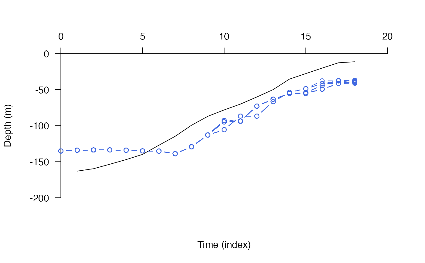
The function returns a plot of the observed and reconstructed depth time series, either for all paths at once (if prompt = FALSE) or each path separately (if prompt = TRUE).

Details

Observed and reconstructed depth time series can differ due to measurement error, which is controlled via the calc_depth_error function in the DC and ACDC algorithms (see dc and acdc).

See also

pf implements the pf algorithm. pf_plot_history visualises particle histories, pf_plot_map creates an overall `probability of use' map from particle histories and pf_simplify processes the outputs into a dataframe of movement paths. pf_plot_1d, pf_plot_2d and pf_plot_3d provide plotting routines for paths. pf_loglik calculates the log-probability of each path.

Author

Edward Lavender

Examples

#### Implement pf() algorithm
# Here, we use pre-defined outputs for speed
paths <- dat_dcpf_paths
archival <- dat_dc$args$archival

#### Example (1): The default implementation
pf_plot_1d(paths, archival)


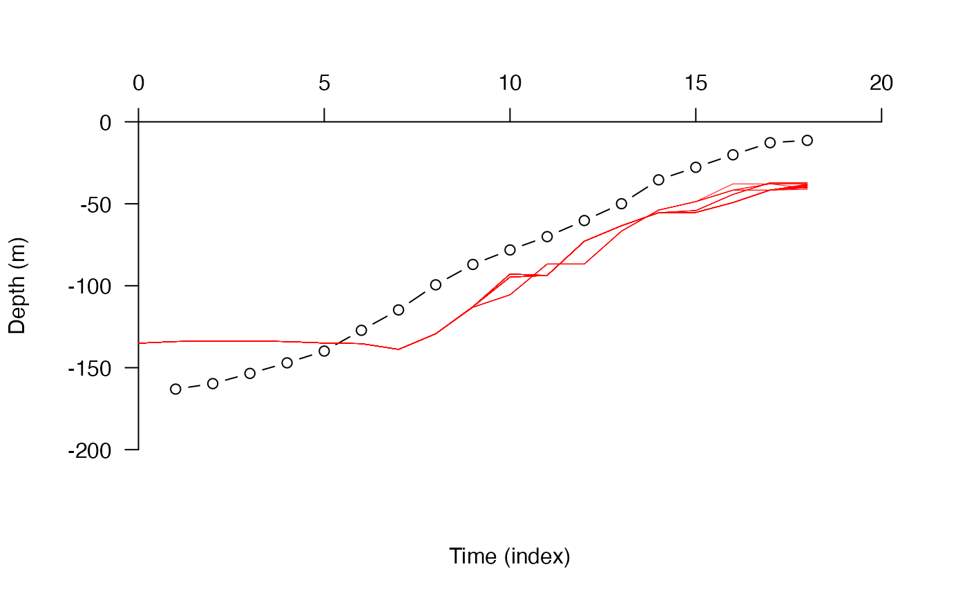
#### Example (2): Plot customisation options, e.g.:
pf_plot_1d(paths, archival, scale = 1, pretty_axis_args = list(side = 1:2))

pf_plot_1d(paths, archival, type = "l")

pf_plot_1d(paths, archival, add_lines = list(col = "red", lwd = 0.5))


#### Example (3): Plot individual comparisons
if (interactive()) {
  pp <- graphics::par(mfrow = c(3, 4))
  pf_plot_1d(paths, depth, prompt = TRUE)
  graphics::par(pp)
}