This function plots the spatiotemporal particle histories from a particle filtering (PF) algorithm (the acoustic-container PF, the depth-contour PF or the acoustic-container depth-contour PF). This produces, for each time step, a map of the individual's possible locations (from the AC, DC or ACDC algorithm), with sampled locations (derived via the particle filtering routine) overlaid.
Arguments
- archive
A
pf_archive-classobject frompf, orpfpluspf_simplifywith thereturn = "archive"argument, that contains particle histories.- time_steps
An integer vector that defines the time steps for which to plot particle histories.
- add_surface
A named list, passed to
pretty_map, to customise the appearance of the surface, which shows the set of possible positions that the individual could have occupied at a given time step (fromac,dcandacdc), on each map.- add_particles
A named list, passed to
pretty_map, to customise the appearance of the particles on each map.- forwards
A logical variable that defines whether or not create plots forwards (i.e., from the first to the last
time_steps) or backwards (i.e., from the last to the firsttime_steps).- prompt
A logical input that defines whether or not to pause between plots (
prompt = TRUE).- ...
Plot customisation arguments passed to
pretty_map.
Value
The function returns a plot, for each time step, of all the possible locations of the individual, with sampled locations overlaid.
See also
pf implements PF. pf_simplify assembles paths from particle histories. pf_plot_map creates an overall `probability of use' map from particle histories. pf_plot_1d, pf_plot_2d and pf_plot_3d provide plotting routines for paths. pf_loglik calculates the log-probability of each path.
pf implements PF. pf_simplify assembles paths from particle histories. pf_plot_history visualises particle histories. pf_plot_1d, pf_plot_2d and pf_plot_3d provide plotting routines for paths. pf_loglik calculates the log-probability of each path.
Examples
#### Implement pf() algorithm
# Here, we use pre-defined outputs for speed
#### Example (1): The default implementation
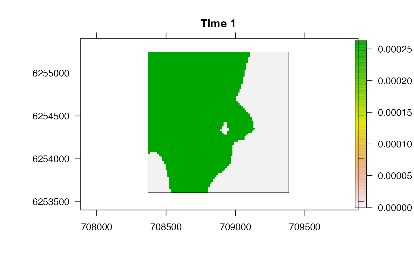
pf_plot_history(dat_dcpf_histories, time_steps = 1)
#> Spatial layers do not have identical CRS strings
#> prettyGraphics::pretty_map() CRS taken as: 'NA'.
 #### Example (2): Plot customisation options, e.g.:
# Customise bathy via add_bathy()
pf_plot_history(dat_dcpf_histories,
time_steps = 1,
add_surface = list(col = c(grDevices::topo.colors(2)))
)
#> Spatial layers do not have identical CRS strings
#> prettyGraphics::pretty_map() CRS taken as: 'NA'.
#### Example (2): Plot customisation options, e.g.:
# Customise bathy via add_bathy()
pf_plot_history(dat_dcpf_histories,
time_steps = 1,
add_surface = list(col = c(grDevices::topo.colors(2)))
)
#> Spatial layers do not have identical CRS strings
#> prettyGraphics::pretty_map() CRS taken as: 'NA'.
 # Customise particles via add_particles
pf_plot_history(dat_dcpf_histories,
time_steps = 1,
add_particles = list(col = "red")
)
#> Spatial layers do not have identical CRS strings
#> prettyGraphics::pretty_map() CRS taken as: 'NA'.
# Customise particles via add_particles
pf_plot_history(dat_dcpf_histories,
time_steps = 1,
add_particles = list(col = "red")
)
#> Spatial layers do not have identical CRS strings
#> prettyGraphics::pretty_map() CRS taken as: 'NA'.
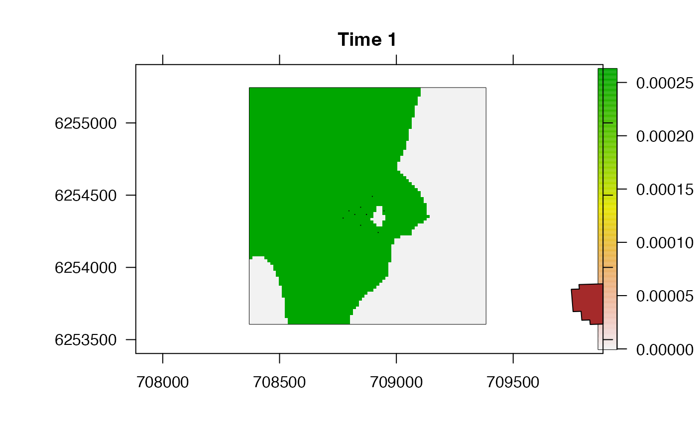
 # Pass other arguments to prettyGraphics::pretty_map() via ...
pf_plot_history(dat_dcpf_histories,
time_steps = 1,
add_polys = list(x = dat_coast, col = "brown"),
crop_spatial = TRUE
)
#> Spatial layers do not have identical CRS strings
#> prettyGraphics::pretty_map() CRS taken as: 'NA'.
# Pass other arguments to prettyGraphics::pretty_map() via ...
pf_plot_history(dat_dcpf_histories,
time_steps = 1,
add_polys = list(x = dat_coast, col = "brown"),
crop_spatial = TRUE
)
#> Spatial layers do not have identical CRS strings
#> prettyGraphics::pretty_map() CRS taken as: 'NA'.
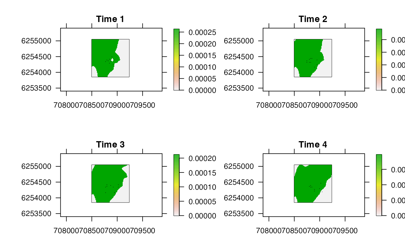
 #### Example (3): Plot multiple time steps
pp <- graphics::par(mfrow = c(2, 2))
pf_plot_history(dat_dcpf_histories, time_steps = 1:4, prompt = FALSE)
#> Spatial layers do not have identical CRS strings
#> prettyGraphics::pretty_map() CRS taken as: 'NA'.
#> Spatial layers do not have identical CRS strings
#> prettyGraphics::pretty_map() CRS taken as: 'NA'.
#> Spatial layers do not have identical CRS strings
#> prettyGraphics::pretty_map() CRS taken as: 'NA'.
#> Spatial layers do not have identical CRS strings
#> prettyGraphics::pretty_map() CRS taken as: 'NA'.
#### Example (3): Plot multiple time steps
pp <- graphics::par(mfrow = c(2, 2))
pf_plot_history(dat_dcpf_histories, time_steps = 1:4, prompt = FALSE)
#> Spatial layers do not have identical CRS strings
#> prettyGraphics::pretty_map() CRS taken as: 'NA'.
#> Spatial layers do not have identical CRS strings
#> prettyGraphics::pretty_map() CRS taken as: 'NA'.
#> Spatial layers do not have identical CRS strings
#> prettyGraphics::pretty_map() CRS taken as: 'NA'.
#> Spatial layers do not have identical CRS strings
#> prettyGraphics::pretty_map() CRS taken as: 'NA'.
 graphics::par(pp)
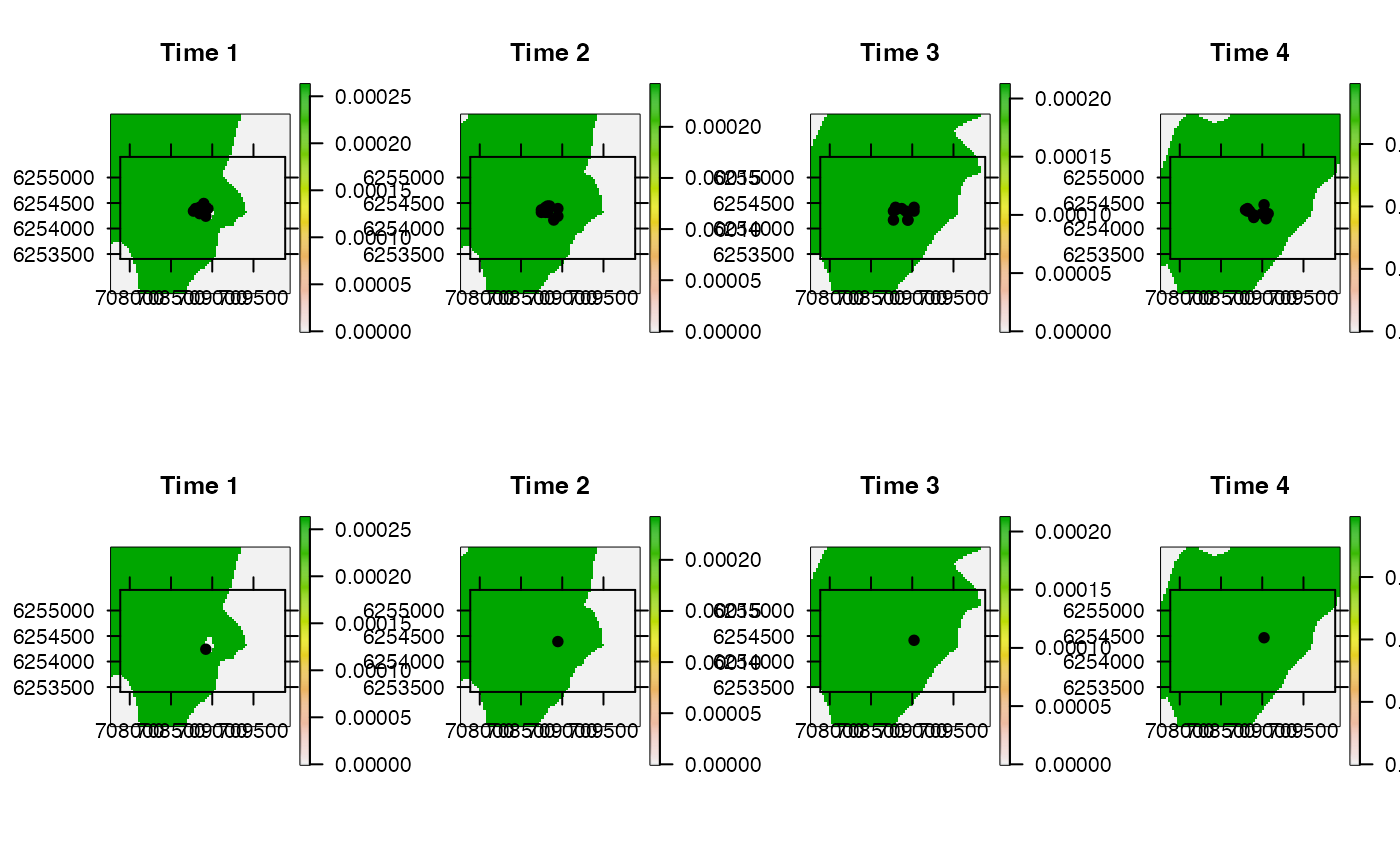
#### Example (4): Compare outputs for sampled versus connected particles
dat_dcpf_histories_connected <-
pf_simplify(dat_dcpf_histories, return = "archive")
#> flapper::pf_simplify() called (@ 2023-08-29 15:45:43)...
#> ... Getting pairwise cell movements based on calc_distance = 'euclid'...
#> ... ... Stepping through time steps to join coordinate pairs...
#> ... ... Identifying connected cells...
#> ... ... Processing connected cells for return = 'archive'...
#> ... flapper::pf_simplify() call completed (@ 2023-08-29 15:45:43) after ~0 minutes.
pp <- graphics::par(mfcol = c(2, 4))
pf_plot_history(dat_dcpf_histories,
time_steps = 1:4,
add_particles = list(pch = 21, bg = "black"),
prompt = FALSE
)
#> Spatial layers do not have identical CRS strings
#> prettyGraphics::pretty_map() CRS taken as: 'NA'.
#> Spatial layers do not have identical CRS strings
#> prettyGraphics::pretty_map() CRS taken as: 'NA'.
#> Spatial layers do not have identical CRS strings
#> prettyGraphics::pretty_map() CRS taken as: 'NA'.
#> Spatial layers do not have identical CRS strings
#> prettyGraphics::pretty_map() CRS taken as: 'NA'.
pf_plot_history(dat_dcpf_histories_connected,
time_steps = 1:4,
add_particles = list(pch = 21, bg = "black"),
prompt = FALSE
)
#> Spatial layers do not have identical CRS strings
#> prettyGraphics::pretty_map() CRS taken as: 'NA'.
#> Spatial layers do not have identical CRS strings
#> prettyGraphics::pretty_map() CRS taken as: 'NA'.
#> Spatial layers do not have identical CRS strings
#> prettyGraphics::pretty_map() CRS taken as: 'NA'.
#> Spatial layers do not have identical CRS strings
#> prettyGraphics::pretty_map() CRS taken as: 'NA'.
graphics::par(pp)
#### Example (4): Compare outputs for sampled versus connected particles
dat_dcpf_histories_connected <-
pf_simplify(dat_dcpf_histories, return = "archive")
#> flapper::pf_simplify() called (@ 2023-08-29 15:45:43)...
#> ... Getting pairwise cell movements based on calc_distance = 'euclid'...
#> ... ... Stepping through time steps to join coordinate pairs...
#> ... ... Identifying connected cells...
#> ... ... Processing connected cells for return = 'archive'...
#> ... flapper::pf_simplify() call completed (@ 2023-08-29 15:45:43) after ~0 minutes.
pp <- graphics::par(mfcol = c(2, 4))
pf_plot_history(dat_dcpf_histories,
time_steps = 1:4,
add_particles = list(pch = 21, bg = "black"),
prompt = FALSE
)
#> Spatial layers do not have identical CRS strings
#> prettyGraphics::pretty_map() CRS taken as: 'NA'.
#> Spatial layers do not have identical CRS strings
#> prettyGraphics::pretty_map() CRS taken as: 'NA'.
#> Spatial layers do not have identical CRS strings
#> prettyGraphics::pretty_map() CRS taken as: 'NA'.
#> Spatial layers do not have identical CRS strings
#> prettyGraphics::pretty_map() CRS taken as: 'NA'.
pf_plot_history(dat_dcpf_histories_connected,
time_steps = 1:4,
add_particles = list(pch = 21, bg = "black"),
prompt = FALSE
)
#> Spatial layers do not have identical CRS strings
#> prettyGraphics::pretty_map() CRS taken as: 'NA'.
#> Spatial layers do not have identical CRS strings
#> prettyGraphics::pretty_map() CRS taken as: 'NA'.
#> Spatial layers do not have identical CRS strings
#> prettyGraphics::pretty_map() CRS taken as: 'NA'.
#> Spatial layers do not have identical CRS strings
#> prettyGraphics::pretty_map() CRS taken as: 'NA'.
 graphics::par(pp)