Movement models

ModelMove is Abstract Type in Patter.jl that groups movement model sub-types, of which instances can be created via an R model_move_*() function.

Usage

model_move_xy(
  .mobility = "750.0",
  .dbn_length = "truncated(Gamma(1, 250.0), upper = 750.0)",
  .dbn_heading = "Uniform(-pi, pi)"
)

model_move_xyz(
  .mobility = "750.0",
  .dbn_length = "truncated(Gamma(1, 250.0), upper = 750.0)",
  .dbn_heading = "Uniform(-pi, pi)",
  .dbn_z = "truncated(Normal(100.0, 250.0), lower = 0.0, upper = 350.0)"
)

model_move_cxy(
  .mobility = "750.0",
  .dbn_length = "truncated(Gamma(1.0, 750.0), upper = 750.0)",
  .dbn_heading_delta = "Normal(0, 0.5)"
)

model_move_cxyz(
  .mobility = "750.0",
  .dbn_length = "truncated(Gamma(1.0, 750.0), upper = 750.0)",
  .dbn_heading_delta = "Normal(0, 0.5)",
  .dbn_z_delta = "Normal(0, 3.5)"
)

Arguments

.mobility, .dbn_length, .dbn_heading, .dbn_heading_delta, .dbn_z, .dbn_z_delta

Character strings that define movement model components:

.mobility—the maximum movement distance between two time steps (m);
.dbn_length—the distribution of step lengths (m);
.dbn_heading—the distribution of headings (rad);
.dbn_heading_delta—the distribution of changes in heading, i.e., turning angle (rad);
.dbn_z—the distribution of depths;
.dbn_z_delta—the distribution of changes in depth;

Value

model_move_*() functions return a character string that defines a ModelMove instance for evaluation in Julia. The class of the output is character plus ModelMove and ModelMoveXY, ModelMoveXYZ, ModelMoveCXY or ModelMoveCXYZ (see plot.ModelMove). If the map (env) does not exist in Julia, an error is thrown.

Model structures

Movement model sub-types are Julia structures that hold the components of movement models. From an R-user perspective, you can think of a ModelMove sub-type as an S4-class-like object, with slots for the components of a movement model. With a movement model instance, we can simulate movements and evaluate the density of movements from one state (location) to another.

The following movement models are built in to Patter.jl:

Random walks (RWs):
- ModelMoveXY
- ModelMoveXYZ
Correlated random walks (CRWs):
- ModelMoveCXY
- ModelMoveCXYZ

See Patter.jl or JuliaCall::julia_help("ModelMove") for the fields of the built-in sub-types. Briefly, all sub-types include:

A map field, that defines the region(s) within which movements are permitted. In R, it is convenient to represent map as a terra::SpatRaster, where NAs define inhospitable habitats (e.g., land). This should made available to Julia ModelMove constructors as env via set_map();
The mobility parameter;
Additional model-specific components (such as fields for the distribution of step lengths and headings in the case of two-dimensional random walks);

In patter, movement models are required:

To simulate movement paths, via sim_path_walk();
To run the particle filter, via pf_filter();
To run the particle smoother, via pf_smoother_two_filter();

In R functions, the movement-model instance is specified via the .model_move argument. This argument expects a character string defining a ModelMove instance that can be evaluated in Julia (that is, a ModelMove constructor). model_move_*() functions are convenience functions for the specification of these constructors for the built-in sub-types. All ModelMove instances contain a map field that defines the region(s) within which movements are permitted. To use a model_move_*() function, the map should be available in Julia as env (see set_map()). The additional components of the movement model are specified via model_move_*() function arguments as character strings of Julia code. Currently implemented model_move_*() functions are:

model_move_xy(), which specifies a RW in X and Y of sub-type ModelMoveXY in terms of the distributions of step lengths and headings;
model_move_xyz(), which specifies a RW in X, Y and Z of sub-type ModelMoveXY in terms of the distributions of step lengths, headings and depths;
model_move_cxy(), which specifies a CRW in X and Y of sub-type ModelMoveXY in terms of the distributions of step lengths and turning angles;
model_move_cxyz(), which specifies a CRW in X, Y and Z of sub-type ModelMoveCXYZ in terms of the distributions of step lengths, turning angles and changes in depth;

See here for the translations of distributions in R (e.g., *norm()) into Julia (e.g., Normal()).

To plot the dimensions of a movement model, see plot.ModelMove. To visualise realisations of a model, see sim_path_walk().

In Julia, ModelMove instances are used to simulate states via Patter.simulate_step(). In the particle smoother, the density of movement from one state to another is evaluated by Patter.logpdf_step(). These are generic functions. Different methods are dispatched according to the input model. For the built-in ModelMove sub-types, corresponding methods for these routines are also built-in. For custom ModelMove sub-types, the methods need to be provided.

To use custom ModelMove sub-types, see ?State.

Model development

For inference, we encourage users to start with simple movement models (such as random walks or correlated random walks) and add complexity iteratively, as required. Movement models should be formulated, and parameterised, using available datasets, domain knowledge and literature. For example:

Lavender et al. (2025). In a study of flapper skate (Dipturus intermedius) movements, we formulated a behavioural-switching correlated random walk movement model. We gauged potential swimming speeds from analyses of movement rates between receivers and vertical activity (via get_mvt_mobility() in flapper). Actual movement speeds can be affected by current speeds and we evaluated these using an ocean model (via fvcom.tbx). We also reviewed information in the literature for related species (from accelerometery, satellite tracking, flow tank experiments and trawl footage). These studies helped to bound our expectations for movement rates in flapper skate, in the absence of direct measurements. Given epistemic uncertainty, we also conducted analyses with 'restrictive' and 'flexible' movement models to analyse algorithm sensitivity.
Lavender et al. (in prep). In a study on lake trout (Salvelinus namaycush), we are leveraging swim-speed information from fine-scale positioning studies, accelerometer measurements and swim-tunnel experiments (plus other datasets such as underwater video) to parameterise our models. For this species, we can visualise the distributions of speed and turning angle measurements (with histograms) and develop data-driven models (e.g., using fitdistrplus::fitdist()).

For the particle filter, movement models must be defined at the resolution of the .timeline (see pf_filter()). For example, if you have a .timeline of two-minute time steps and a simple random walk, the distribution of step lengths (m) and headings (rad) should be defined for a two-minute time step (see model_move_xy()). All movements are truncated by the .mobility parameter. This is the maximum possible movement distance in the time between two time steps. Set .mobility based on the considerations above. Where necessary, you should also account for the discretisation errors in the timing of observations (e.g., see assemble_acoustics()). Since .mobility affects the tail of the distribution, the exact value of .mobility can be relatively unimportant, providing it is large enough. We recommend erring on the side of flexibility in cases of uncertainty.

Note that model formulation and parameterisation can be an iterative process:

Develop initial model and observation models, drawing on available datasets, domain knowledge and literature;
Perform inference, using pf_filter();
Evaluate convergence;
In cases of convergence failures, re-evaluate the model(s) and try again;
Where necessary, run the algorithms with more restrictive or flexible models to analyse sensitivity;

For advice for your study system, please raise an issue on GitHub.

Author

Edward Lavender

Examples

if (patter_run(.julia = TRUE, .geospatial = TRUE)) {

  library(data.table)
  library(JuliaCall)

  #### Connect to Julia
  julia_connect()
  set_seed()

  #### Define the `map`
  # `map` is the region within which movements are permitted
  # In `R`, we represent this as a `SpatRaster`
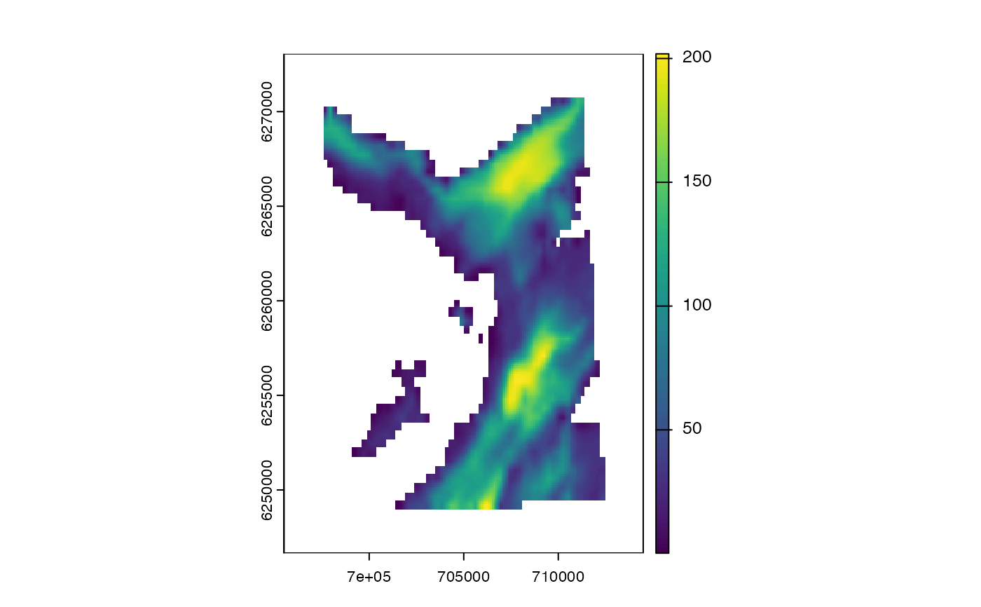
  # Here, we have a bathymetry `SpatRaster` for the west coast of Scotland:
  # * NaNs define regions into which movement is not permitted
  # * (i.e., on land, in the case of aquatic animals)
  map <- dat_gebco()

  # Using `set_map()` makes the map available as a object called 'env' in `Julia`
  # > This is required as a component of all movement models
  set_map(map)

  #### Example (1a): Use `model_move_xy()` with default options
  # `model_move_*()` functions simply return a character string of Julia code
  # (Downstream functions can evaluate this code, as shown below)
  model_move_xy()

  #### Example (1b): Customise `model_move_xy()`
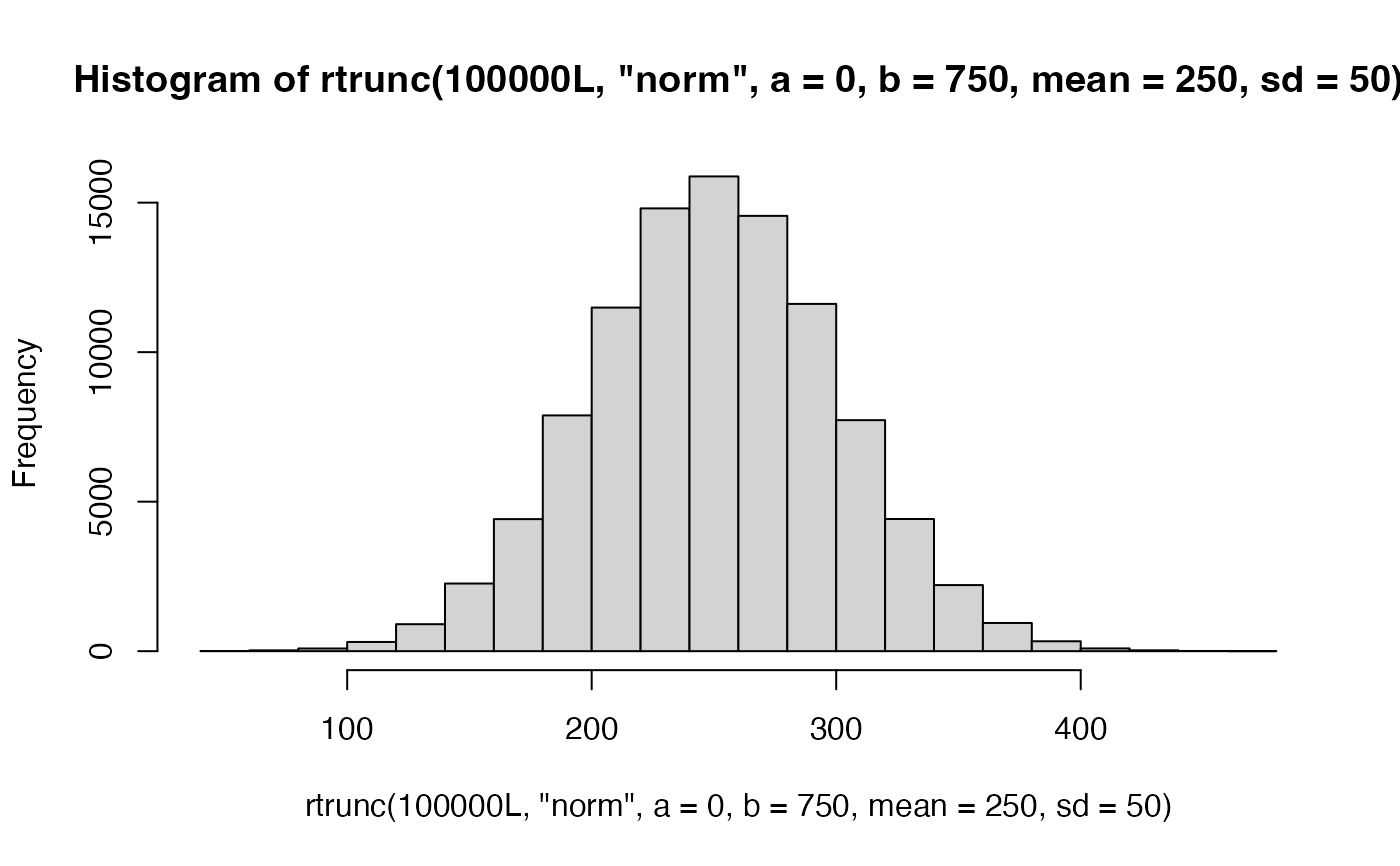
  # Use a truncated normal distribution for step lengths:
  model_move_xy(.mobility = "750.0",
                .dbn_length = "truncated(Normal(250, 50), lower = 0.0, upper = 750.0)")
  # Use an exponential distribution for step lengths
  model_move_xy(.mobility = "750.0",
                .dbn_length = "truncated(Exponential(0.01), upper = 750.0)")
  # Use a biased random walk
  model_move_xy(.dbn_heading = "VonMises(0, 1)")
  # Get help on a distribution in Julia:
  julia_help("Exponential")

  #### Example (2): Use `model_move_xyz()`
  # Use default options
  model_move_xyz()
  # Customise model components
  model_move_xyz(.mobility = "750.0",
                 .dbn_length = "truncated(Exponential(0.01), upper = 750.0)",
                 .dbn_z = "truncated(Gamma(1.0, 250.0), lower = 0.0, upper = 350.0)")

  #### Example (3): Use `model_move_cxy()`
  # Use default options
  model_move_cxy()
  # Customise model components
  model_move_cxy(.mobility = "750.0",
                 .dbn_length = "truncated(Normal(250, 50), lower = 0.0, upper = 750.0)",
                 .dbn_heading_delta = "Normal(0, 0.25)")

  #### Example (4): Use `model_move_cxyz()`
  # Use default options
  model_move_cxyz()
  # Customise model components
  model_move_cxyz(.mobility = "750.0",
                  .dbn_length = "truncated(Normal(250, 50), lower = 0.0, upper = 750.0)",
                  .dbn_heading_delta = "Normal(0, 0.25)",
                  .dbn_z_delta = "Normal(0, 2.5)")

  #### Example (4): Visualise movement model component distributions
  # See `?plot.ModelMove`
  plot(model_move_xy())

  #### Example (5): Visualise movement model realisations (trajectories)
  # See `?sim_path_walk`
  # Define a timeline for the simulation
  timeline <- seq(as.POSIXct("2016-01-01", tz = "UTC"),
                  length.out = 1000L, by = "2 mins")
  # Define an initial location
  x <- 708212.6
  y <- 6251684
  origin <- data.table(map_value = terra::extract(map, cbind(x, y))[1, 1],
                       x = x, y = y)
  # Collect essential arguments for `sim_path_walk()`
  args <- list(.map = map,
               .xinit = origin,
               .timeline = timeline,
               .state = "StateXY",
               .n_path = 2L, .one_page = FALSE)
  # Compare different movement models via `sim_path_walk()`
  pp <- par(mfrow = c(2, 2))
  args$.model_move <- model_move_xy()
  do.call(sim_path_walk, args)
  args$.model_move <- model_move_xy(.dbn_heading = "VonMises(0.1, 0.1)")
  do.call(sim_path_walk, args)
  par(pp)

  #### Example (6): Use movement models in the particle filter
  # See `?pf_filter()`

  #### Example (7): Use custom movement model types
  # Patter contains multiple built-in `State` and `ModelMove` sub-types that you can use
  # ... (with custom parameters) simulate movements and for particle filtering.
  # See the help file for `?State` to use a new sub-type.

}
#> `patter::julia_connect()` called @ 2025-04-22 09:30:02... 
#> ... Running `Julia` setup via `JuliaCall::julia_setup()`... 
#> Julia version 1.11.5 at location /Users/lavended/.julia/juliaup/julia-1.11.5+0.aarch64.apple.darwin14/bin will be used.
#> Loading setup script for JuliaCall...
#> Finish loading setup script for JuliaCall.
#> ... Validating Julia installation... 
#> ... Setting up Julia project... 
#> ... Handling dependencies... 
#> ... `Julia` set up with 11 thread(s). 
#> `patter::julia_connect()` call ended @ 2025-04-22 09:30:11 (duration: ~9 sec(s)). 
#> ```
#> Exponential(θ)
#> ```
#> 
#> The *Exponential distribution* with scale parameter `θ` has probability density function
#> 
#> $$
#> f(x; \theta) = \frac{1}{\theta} e^{-\frac{x}{\theta}}, \quad x > 0
#> $$
#> 
#> ```julia
#> Exponential()      # Exponential distribution with unit scale, i.e. Exponential(1)
#> Exponential(θ)     # Exponential distribution with scale θ
#> 
#> params(d)          # Get the parameters, i.e. (θ,)
#> scale(d)           # Get the scale parameter, i.e. θ
#> rate(d)            # Get the rate parameter, i.e. 1 / θ
#> ```
#> 
#> External links
#> 
#>   * [Exponential distribution on Wikipedia](http://en.wikipedia.org/wiki/Exponential_distribution)

#> Warning: Use `seq.POSIXt()` with `from`, `to` and `by` rather than `length.out` for faster handling of time stamps.
#> Warning: Use `seq.POSIXt()` with `from`, `to` and `by` rather than `length.out` for faster handling of time stamps.