This function runs the particle filter. The filter samples possible states (typically locations, termed particles) of an animal at each time point given the data up to (and including) that time point and a movement model.
Usage
pf_filter(
  .timeline,
  .state = "StateXY",
  .xinit = NULL,
  .model_move = model_move_xy(),
  .yobs,
  .n_move = 100000L,
  .n_particle = 1000L,
  .n_resample = as.numeric(.n_particle),
  .t_resample = NULL,
  .n_record = 1000L,
  .n_iter = 1L,
  .direction = c("forward", "backward"),
  .batch = NULL,
  .collect = TRUE,
  .progress = julia_progress(),
  .verbose = getOption("patter.verbose")
)
Arguments
- .timeline
A
POSIXctvector of regularly spaced time stamps that defines the timeline for the simulation. Here,.timelineis used to:Define the time steps of the simulation;
- .state, .xinit
Arguments used to simulate initial states.
.state—Acharacterthat defines theStatesub-type;.xinit—NULLor adata.table::data.tablethat defines the initial states for the simulation;
- .model_move, .n_move
The movement model.
.model_move—Acharacterstring that defines the movement model (seeModelMove);.n_move—Anintegerthat defines the number of attempts to find a legal move;
- .yobs
The observations. Acceptable inputs are:
A named
listof formatted datasets, one for each data type (seeglossary);An empty
list, to run the filter without observations;missing, if the datasets are already available in theJuliasession (from a previous run ofpf_filter()) and you want to re-run the filter without the penalty of re-exporting the observations;
- .n_particle
An
integerthat defines the number of particles.- .n_resample, .t_resample
Resampling options.
.n_resampleis an adoublethat defines the effective sample size (ESS) at which to re-sample particles;.t_resampleisNULLor aninteger/integervector that defines the time steps at which to resample particles, regardless of the ESS;
Guidance:
To resample at every time step, set
.n_resample = as.numeric(.n_particle)(default) or.t_resample = 1:length(.timeline);To only resample at selected time steps, set
.t_resampleas required and set.n_resample > as.numeric(.n_particle);To only resample based on ESS, set
.t_resample = NULLand.n_resampleas required;
- .n_record
An
integerthat defines the number of recorded particles at each time step.- .n_iter
An
integerthat defines the number of iterations of the filter.- .direction
A
characterstring that defines the direction of the filter:"forward"runs the filter from.timeline[1]:.timeline[length(.timeline)];"backward"runs the filter from.timeline[length(.timeline)]:.timeline[1];
- .batch
(optional) Batching controls:
Use
NULLto retain all particles for the whole.timeline(.n_recordparticles at each time step) in memory;Use
charactervector of.jld2file paths to write particles in sequential batches to file (asJuliaMatrix{<:State}objects); for example:./fwd-1.jld2, ./fwd-2.jld2, ...if.direction = "forward";./bwd-1.jld2, ./bwd-2.jld2, ...if.direction = "backward;
If specified,
.batchis sorted alphanumerically (inJulia) such that 'lower' batches (e.g.,./fwd-1.jld2,./bwd-1.jld2) align with the start of the.timelineand 'higher' batches (e.g.,./fwd-3.jld2,./bwd-3.jld2) align with the end of the.timeline(irrespective of.direction). For smoothing, the same number of batches must be used for both filter runs (seepf_smoother_two_filter()).This option is designed to reduce memory demand (especially on clusters). Larger numbers of batches reduce memory demand, but incur the speed penalty of writing particles to disk. When there are only a handful of batches, this should be negligible. For examples of this argument in action, see
pf_smoother_two_filter().- .collect
A
logicalvariable that defines whether or not to collect outputs from theJuliasession inR.- .progress
Progress controls (see
patter-progressfor supported options). If enabled, one progress bar is shown for each.batch.- .verbose
User output control (see
patter-progressfor supported options).
Value
Patter.particle_filter() creates a NamedTuple in the Julia session (named pfwd or pbwd depending on .direction). If .batch = NULL, the NamedTuple contains particles (states) ; otherwise, the states element is nothing and states are written to .jld2 files (as variables named xfwd or xbwd). If .collect = TRUE, pf_filter() collects the outputs in R as a pf_particles object (the states element is NULL is .batch is used). Otherwise, invisible(NULL) is returned.
Overview
The particle filter iterates over time steps, simulating states (termed 'particles') that are consistent with the preceding data and a movement model at each time step.
A raster map of study area must be exported to Julia for this function (see set_map()).
The initial states for the algorithm are defined by .xinit or simulated via Patter.simulate_states_init(). The word 'state' typically means location but may include additional parameters. If the initial state of the animal is known, it should be supplied via .xinit. Otherwise, Patter.simulate_states_init() samples .n_particle initial coordinates from .map (via Patter.coords_init()), which are then translated into a DataFrame of states (that is, .xinit, via Patter.states_init()). The regions on the map from which initial coordinates are sampled can be restricted by the observations (.yobs) and other parameters. For automated handling of custom states and observation models at this stage, custom Patter.map_init and Patter.states_init methods are required (see the Details for Patter.simulate_states_init()).
The filter comprises three stages:
A movement step, in which we simulate possible states (particles) for the individual (for time steps 2, ..., T).
A weights step, in which we calculate particle weights from the log-likelihood of the data at each particle.
A re-sampling step, in which we optionally re-sample valid states using the weights.
The time complexity of the algorithm is \(O(TN)\).
The filter is implemented by the Julia function Patter.particle_filter().
To multi-thread movement and likelihood evaluations, set the number of threads via julia_connect().
The filter record .n_record particles in memory at each time step. If batch is provided, the .timeline is split into length(.batch) batches. The filter still moves along the whole .timeline, but only records the particles for the current batch in memory. At the end of each batch, the particles for that batch are written to file. This reduces total memory demand.
See Patter.particle_filter() or JuliaCall::julia_help("particle_filter") for further information.
Algorithms
This is highly flexible routine for the reconstruction of the possible locations of an individual through time, given the data up to that time point. By modifying the observation models, it is straightforward to implement the ACPF, DCPF and ACDCPF algorithms introduced by Lavender et al. (2023) for reconstructing animal movements in passive acoustic telemetry systems using (a) acoustic time series, (b) archival time series and (c) acoustic and archival time series. pf_filter() thus replaces (and enhances) the flapper::ac(), flapper::dc(), flapper::acdc() and flapper::pf() functions.
See also
Particle filters and smoothers sample states (particles) that represent the possible locations of an individual through time, accounting for all data and the individual's movement.
To simulate artificial datasets, see
sim_*()functions (especiallysim_path_walk(),sim_array()andsim_observations()).To assemble real-world datasets for the filter, see
assemble_*()functions.pf_filter()runs the filter:To run particle smoothing, use
pf_smoother_two_filter().To map emergent patterns of space use, use a
map_*()function (such asmap_pou(),map_dens()andmap_hr()).
Examples
if (patter_run(.julia = TRUE, .geospatial = TRUE)) {
library(data.table)
library(dtplyr)
library(dplyr, warn.conflicts = FALSE)
library(glue)
#### Julia set up
julia_connect()
set_seed()
#### Define study period
# The resolution of the timeline defines the resolution of the simulation
timeline <- seq(as.POSIXct("2016-01-01", tz = "UTC"),
as.POSIXct("2016-01-01 03:18:00", tz = "UTC"),
by = "2 mins")
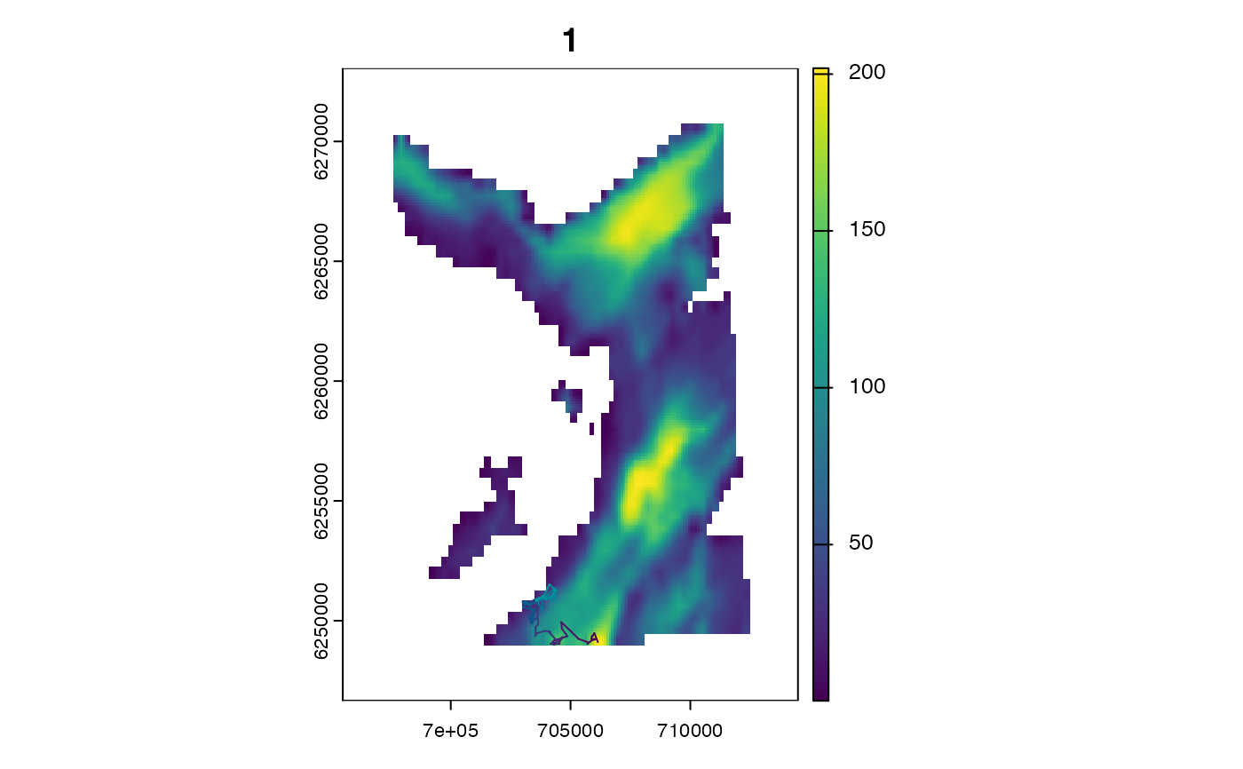
#### Define study area
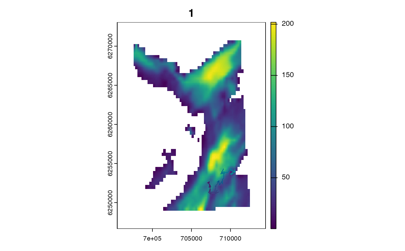
# `map` is a SpatRaster that defines the region within which movements are permitted
# Here, we consider the movements of an aquatic animal in Scotland
# ... `map` represents the bathymetry in the relevant region
# Use `set_map()` to export the map to `Julia`
map <- dat_gebco()
terra::plot(map)
set_map(map)
#### --------------------------------------------------
#### Simulation-based workflow
#### Scenario
# We have studied the movements of flapper skate off the west coast of Scotland.
# We have collected acoustic detections at receivers and depth time series.
# Here, we simulate movements and acoustic/archival observations arising from movements.
# We then apply particle filtering to the 'observations' to reconstruct
# ... simulated movements.
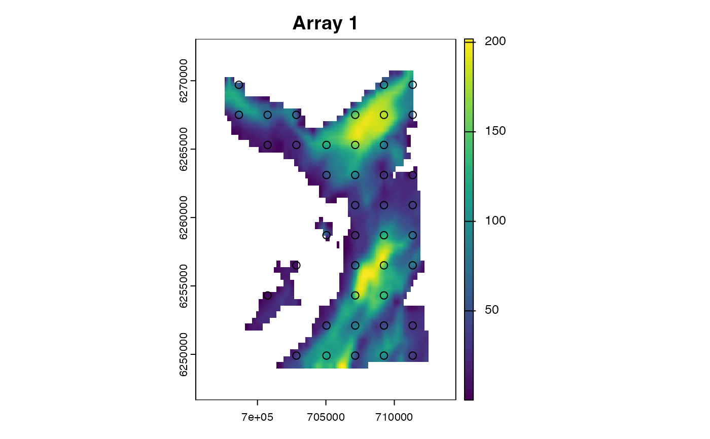
#### Simulate an acoustic array
moorings <- sim_array(.map = map,
.timeline = timeline,
.n_receiver = 100L)
# `moorings` includes the following default observation model parameters
# * These describe how detection probability declines with distance from a receiver
# * These are the parameters of the `ModelObsAcousticLogisTrunc` observation model
a <- moorings$receiver_alpha[1]
b <- moorings$receiver_beta[1]
g <- moorings$receiver_gamma[1]
d <- seq(1, 1000, by = 1)
plot(d, ifelse(d <= g, plogis(a * b * d), 0),
ylab = "Detection probability",
xlab = "Distance (m)",
type = "l")
#### Simulate a movement path
# Define `State` sub-type
# > We will consider the animal's movement in two-dimensions (x, y)
state <- "StateXY"
# Define the maximum moveable distance (m) between two time steps
mobility <- 750
# Define the movement model
# > We consider a two-dimensional random walk
model_move <-
model_move_xy(.mobility = "750.0",
.dbn_length = "truncated(Gamma(1, 250.0), upper = 750.0)",
.dbn_heading = "Uniform(-pi, pi)")
# Simulate a path
paths <- sim_path_walk(.map = map,
.timeline = timeline,
.state = state,
.model_move = model_move)
#### Simulate observations
# Define observation model(s)
# * We simulate acoustic observations and depth time series
# * Acoustic observations are simulated according to `ModelObsAcousticLogisTrunc`
# * Depth observations are simulated according to `ModelObsDepthUniformSeabed`
# Define a `list` of parameters for the observation models
# (See `?ModelObs` for details)
pars_1 <-
moorings |>
select(sensor_id = "receiver_id", "receiver_x", "receiver_y",
"receiver_alpha", "receiver_beta", "receiver_gamma") |>
as.data.table()
pars_2 <- data.table(sensor_id = 1L,
depth_shallow_eps = 10,
depth_deep_eps = 10)
model_obs <- list(ModelObsAcousticLogisTrunc = pars_1,
ModelObsDepthUniformSeabed = pars_2)
# Simulate observational datasets
obs <- sim_observations(.timeline = timeline,
.model_obs = model_obs)
summary(obs)
head(obs$ModelObsAcousticLogisTrunc[[1]])
head(obs$ModelObsDepthUniformSeabed[[1]])
# Identify detections
detections <-
obs$ModelObsAcousticLogisTrunc[[1]] |>
filter(obs == 1L) |>
as.data.table()
# Collate datasets for filter
# > This requires a list of datasets, one for each data type
# > We could also include acoustic containers here for efficiency (see below)
yobs <- list(ModelObsAcousticLogisTrunc = obs$ModelObsAcousticLogisTrunc[[1]],
ModelObsDepthUniformSeabed = obs$ModelObsDepthUniformSeabed[[1]])
#### Example (1): Run the filter using the default options
fwd <- pf_filter(.timeline = timeline,
.state = state,
.xinit = NULL,
.model_move = model_move,
.yobs = yobs,
.n_particle = 1e4L,
.direction = "forward")
## Output object structure:
# The function returns a `pf_particles` list:
class(fwd)
summary(fwd)
# `states` is a [`data.table::data.table`] of particles:
fwd$states
# `diagnostics` is a [`data.table::data.table`] of filter diagnostics
fwd$diagnostics
# fwd$callstats is a [`data.table::data.table`] of call statistics
fwd$callstats
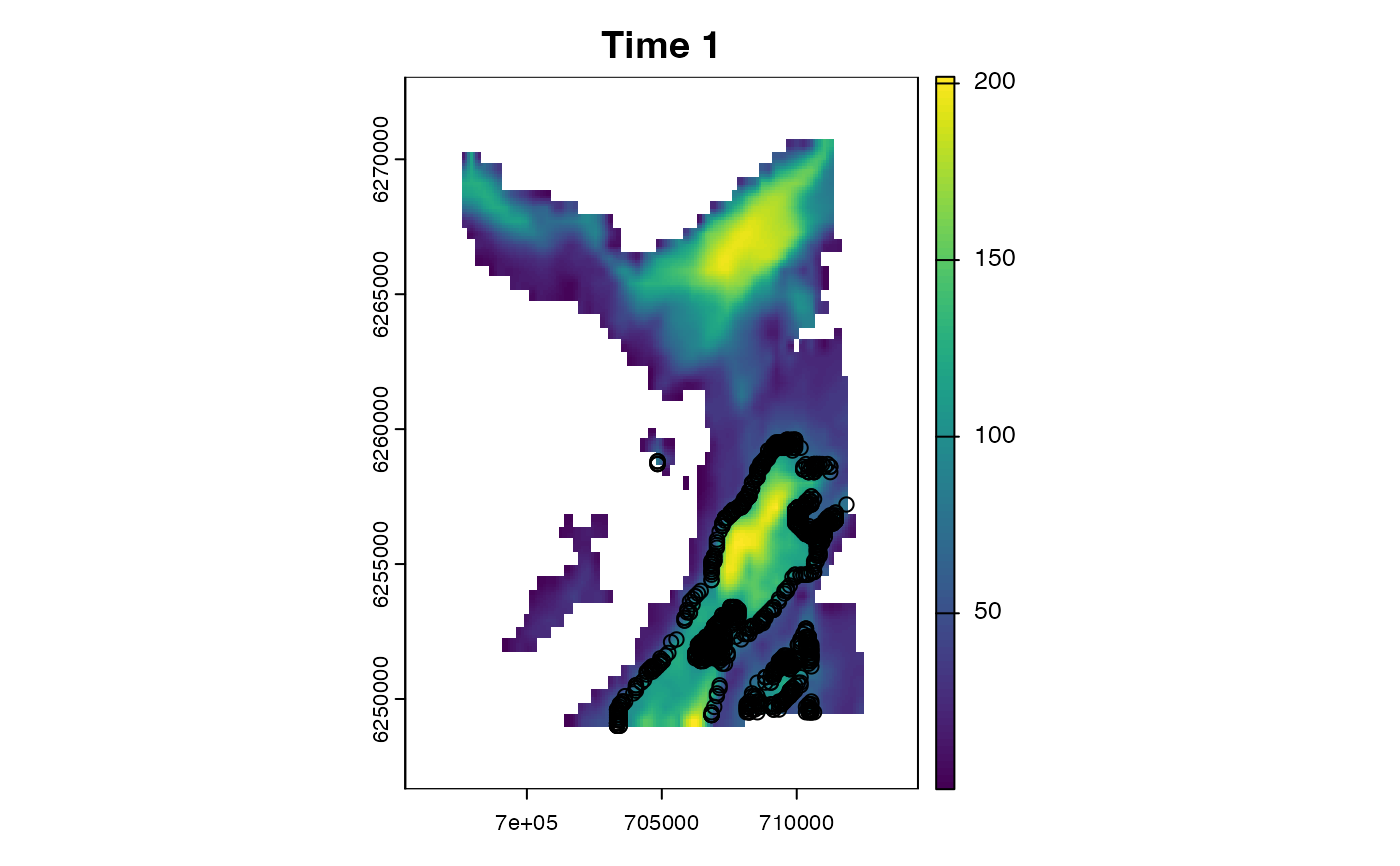
## Map output states:
# Map particle coordinates
plot_xyt(.map = map, .coord = fwd$states, .steps = 1L)
# Map a utilisation distribution
# * Use `.sigma = spatstat.explore::bw.diggle()` for CV bandwidth estimate
map_dens(.map = map,
.coord = fwd$states)
## Analyse filter diagnostics
# `maxlp` is the maximum log-posterior at each time step
# > exp(fwd$diagnostics$maxlp) = the highest likelihood score at each time step (0-1)
# > This should not be too low!
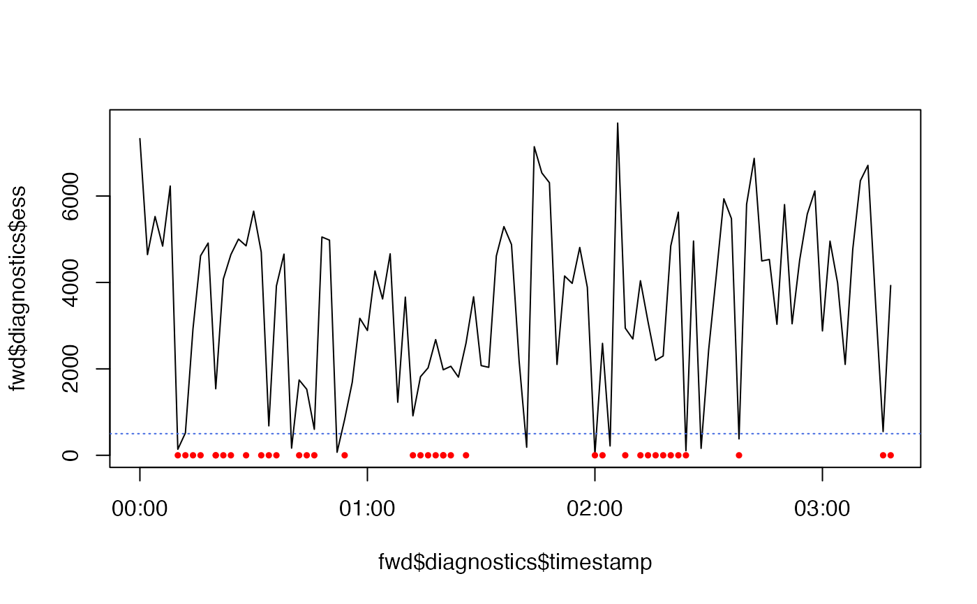
plot(fwd$diagnostics$timestamp, fwd$diagnostics$maxlp, type = "l")
# `ess` is the effective sample size
# > For a 2D distribution, >= 500 particles at each time step should be sufficient
# > But we often have a low ESS at the moment of a detection
# > If this is too low, we can trying boosting `.n_particle`
plot(fwd$diagnostics$timestamp, fwd$diagnostics$ess, type = "l")
points(detections$timestamp, rep(0, nrow(detections)),
pch = 21, col = "red", bg = "red", cex = 0.5)
abline(h = 500, col = "royalblue", lty = 3)
#### Example (2): Customise initial states for the filter
# Option (A): Mark the known starting location on `.map`
# > Initial states are automatically sampled from `.map`
# > We have to reset the initial map in Julia
# > Use set_map with .as_Raster = TRUE and .as_GeoArray = FALSE
# > (After the example, we reset the map for later examples)
origin <- terra::setValues(map, NA)
cell <- terra::cellFromXY(map, cbind(paths$x[1], paths$y[1]))
origin[cell] <- paths$map_value[1]
set_map(.x = origin, .as_Raster = TRUE, .as_GeoArray = FALSE)
fwd <- pf_filter(.timeline = timeline,
.state = state,
.xinit = NULL,
.yobs = yobs,
.model_move = model_move,
.n_particle = 1e4L)
set_map(map, .as_Raster = TRUE, .as_GeoArray = FALSE)
# Option (B): Specify `.xinit` manually
# > `.xinit` is resampled, as required, to generate `.n_particle` initial states
xinit <- data.table(map_value = paths$map_value[1], x = paths$x[1], y = paths$y[1])
fwd <- pf_filter(.timeline = timeline,
.state = state,
.xinit = xinit,
.yobs = yobs,
.model_move = model_move,
.n_particle = 1e4L)
#### Example (3): Customise selected settings
# Boost the number of particles
fwd <- pf_filter(.timeline = timeline,
.state = state,
.xinit = xinit,
.yobs = yobs,
.model_move = model_move,
.n_particle = 1.5e4L)
# Change the threshold ESS for resampling
fwd <- pf_filter(.timeline = timeline,
.state = state,
.xinit = xinit,
.yobs = yobs,
.model_move = model_move,
.n_particle = 1.5e4L,
.n_resample = 1000L)
# Force resampling at selected time steps
# * Other time steps are resampled if ESS < .n_resample
fwd <- pf_filter(.timeline = timeline,
.state = state,
.xinit = xinit,
.yobs = yobs,
.model_move = model_move,
.t_resample = which(timeline %in% detections$timestamp),
.n_particle = 1.5e4L,
.n_resample = 1000L)
# Change the number of particles retained in memory
fwd <- pf_filter(.timeline = timeline,
.state = state,
.xinit = xinit,
.yobs = yobs,
.model_move = model_move,
.n_particle = 1.5e4L,
.n_record = 2000L)
#### Example (2): Run the filter backwards
# (A forward and backward run is required for the two-filter smoother)
fwd <- pf_filter(.timeline = timeline,
.state = state,
.xinit = NULL,
.yobs = yobs,
.model_move = model_move,
.n_particle = 1e4L,
.direction = "backward")
#### --------------------------------------------------
#### Real-world examples
#### Assemble datasets
# Define datasets for a selected animal
# > Here, we consider detections and depth time series from an example flapper skate
individual_id <- NULL
det <- dat_detections[individual_id == 25L, ][, individual_id := NULL]
arc <- dat_archival[individual_id == 25L, ][, individual_id := NULL]
# Define a timeline
# * We can do this manually or use the observations to define a timeline:
timeline <- assemble_timeline(list(det, arc), .step = "2 mins", .trim = TRUE)
timeline <- timeline[1:1440]
range(timeline)
# Assemble a timeline of acoustic observations (0, 1) and model parameters
# * The default acoustic observation model parameters are taken from `.moorings`
acoustics <- assemble_acoustics(.timeline = timeline,
.detections = det,
.moorings = dat_moorings)
# Assemble corresponding acoustic containers
# * This is recommended with acoustic observations
# * Note this dataset is direction specific (see below)
containers <- assemble_acoustics_containers(.timeline = timeline,
.acoustics = acoustics,
.mobility = mobility)
# Assemble a timeline of archival observations and model parameters
# * Here, we include model parameters for `ModelObsDepthNormalTruncSeabed`
archival <- assemble_archival(.timeline = timeline,
.archival =
arc |>
rename(obs = depth) |>
mutate(depth_sigma = 50,
depth_deep_eps = 20))
# Define the .yobs list for each run of the particle filter
yobs_fwd <- list(ModelObsAcousticLogisTrunc = acoustics,
ModelObsContainer = containers$forward,
ModelObsDepthNormalTruncSeabed = archival)
yobs_bwd <- list(ModelObsAcousticLogisTrunc = acoustics,
ModelObsContainer = containers$backward,
ModelObsDepthNormalTruncSeabed = archival)
#### Visualise realisations of the movement model (the prior)
# We will use the same movement model as in previous examples
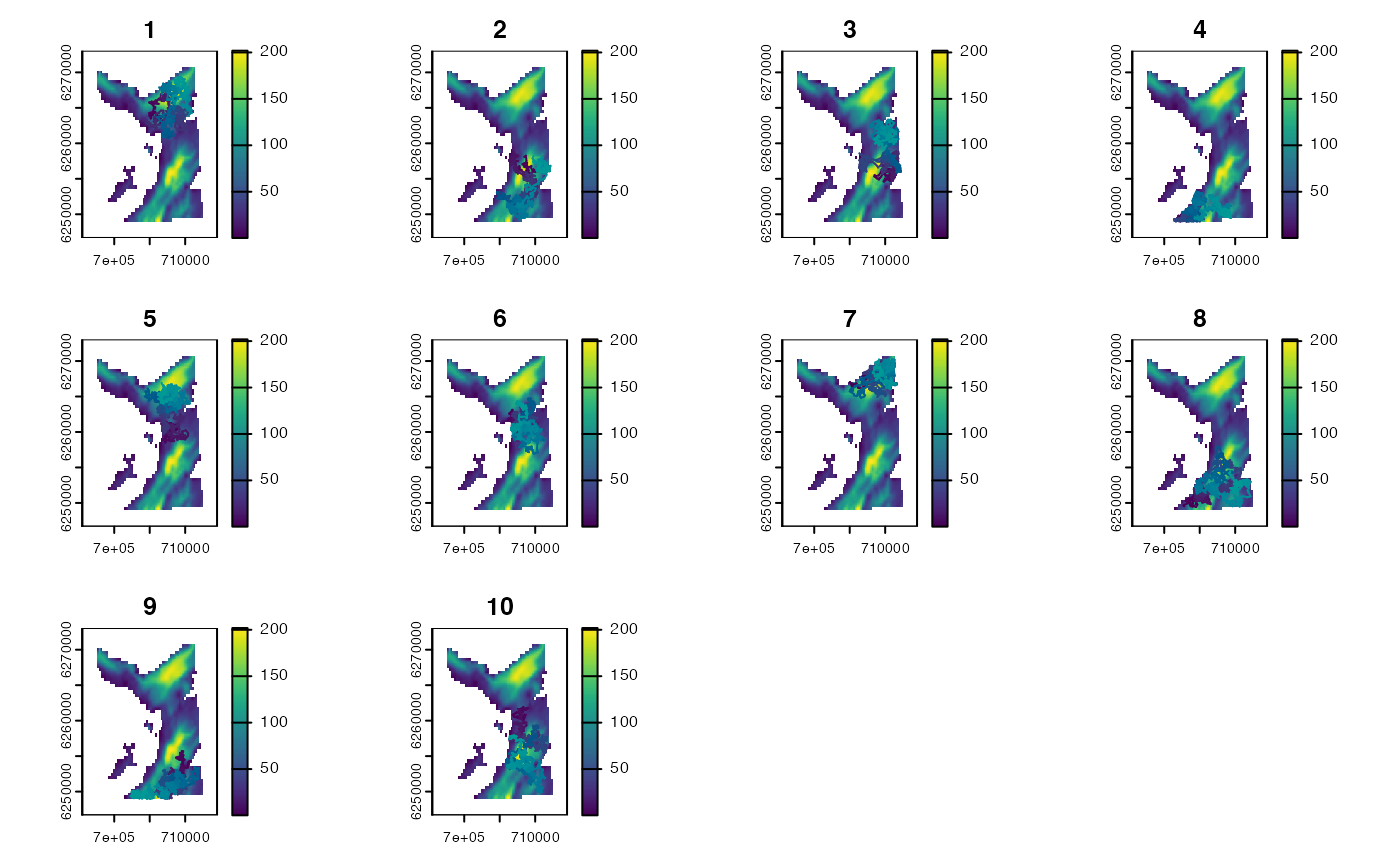
sim_path_walk(.map = map,
.timeline = timeline,
.state = state,
.model_move = model_move,
.n_path = 10L, .one_page = TRUE)
#### Example (1): Run filter forwards
fwd <- pf_filter(.timeline = timeline,
.state = state,
.yobs = yobs_fwd,
.model_move = model_move)
#### Example (2): Run the filter backwards
bwd <- pf_filter(.timeline = timeline,
.state = state,
.yobs = yobs_bwd,
.model_move = model_move,
.direction = "backward")
#### --------------------------------------------------
#### Joint inference of states and static parameters
if (patter_run_expensive()) {
# This example shows how we can infer both states and static parameters:
# * States are our latent locations;
# * Static parameters are the parameters in the movement and observation models;
# For illustration, we'll use simulated data:
# * We consider a passive acoustic telemetry system;
# * The movement model is a Gaussian random walk;
# * The standard deviation of the Gaussian distribution is the 'diffusivity';
# * The observation model is a Bernoulli model for acoustic detections/non-detections;
# Using simulated data, we'll pretend we don't know the movement 'diffusivity':
# * For simplicity, we'll assume we know the other parameters;
# * We'll attempt to estimate the true diffusivity from multiple runs;
# We show how to use the filter log-likelihood score to estimate parameters via:
# * grid-search;
# * maximum likelihood optimisation;
# * Bayesian inference;
# We recommend a simulation analysis like this before real-world analyses:
# * Follow the example below;
# * For your study system and species, simulate observations;
# * Examine whether you have sufficient information to estimate parameters;
# Beware that the log-likelihood value from the filter is 'noisy':
# * This can create all kinds of issues with optimisation & sampling;
# * You should check the sensitivity of the results with regard to the noise;
# * I.e., Re-run the routines a few times to check result consistency;
# Note also that parameter estimation can be computationally expensive:
# * We should select an appropriate inference procedure depending on filter cost;
# * Compromises may be required;
# * We may assume some static parameters are known;
# * We may estimate other parameters for one or two individuals with good data;
# * We may use best-guess parameters + sensitivity analysis;
# * This example just provides a minimal workflow;
#### Define study system
# Define study timeline
timeline <- seq(as.POSIXct("2016-01-01", tz = "UTC"),
as.POSIXct("2016-01-01 03:18:00", tz = "UTC"),
by = "2 mins")
# Define study area
map <- dat_gebco()
set_map(map)
#### Simulate a movement path
# Define movement model
# * `theta` is the movement 'diffusivity'
# * We will attempt to estimate this parameter
state <- "StateXY"
theta <- 250.0
mobility <- 750
model_move <-
model_move_xy(.mobility = mobility,
.dbn_length = glue("truncated(Normal(0, {theta}),
lower = 0.0, upper = {mobility})"),
.dbn_heading = "Uniform(-pi, pi)")
# Simulate a path
path <- sim_path_walk(.map = map,
.timeline = timeline,
.state = state,
.model_move = model_move)
#### Simulate observations
# Simulate array (using default parameters)
# * Note we simulate a dense, regular array here
# * With real-world array designs, there may be less information available
moorings <- sim_array(.map = map,
.timeline = timeline,
.arrangement = "regular",
.n_receiver = 100L)
# Collate observation model parameters
model_obs <- model_obs_acoustic_logis_trunc(moorings)
# Simulate observations arising from path
obs <- sim_observations(.timeline = timeline,
.model_obs = model_obs)
acoustics <- obs$ModelObsAcousticLogisTrunc[[1]]
# (optional) Compute containers
containers <- assemble_acoustics_containers(.timeline = timeline,
.acoustics = acoustics,
.mobility = mobility,
.map = map)
# Collate observations for forward filter
yobs_fwd <-
list(ModelObsAcousticLogisTrunc = obs$ModelObsAcousticLogisTrunc[[1]],
ModelObsContainer = containers$forward)
#### Prepare to estimate the diffusivity using the observations
# i) Visualise movement models with different standard deviations
# > This gives us a feel for how we should constrain the estimation process
# > (if we didn't know the true parameter values)
pp <- par(mfrow = c(3, 3))
thetas <- seq(100, 500, by = 50)
cl_lapply(thetas, function(theta) {
plot(model_move_xy(.mobility = mobility,
.dbn_length = glue::glue("truncated(Normal(0, {theta}),
lower = 0.0, upper = {mobility})"),
.dbn_heading = "Uniform(-pi, pi)"),
.panel_length = list(main = theta, font = 2),
.panel_heading = NULL,
.par = NULL)
})
par(pp)
# ii) Define a function that computes the log-likelihood given input parameters
# * `theta` denotes a parameter/parameter vector
# * (In this case, it is standard deviation in the movement model)
pf_filter_loglik <- function(theta) {
# (safety check) The movement standard deviation cannot be negative
if (theta < 0) {
return(-Inf)
}
# Instantiate movement model
model_move <-
model_move_xy(.mobility = mobility,
.dbn_length = glue::glue("truncated(Normal(0, {theta}),
lower = 0.0, upper = {mobility})"),
.dbn_heading = "Uniform(-pi, pi)")
# Run filter
# * Large .n_particle reduces noise in the likelihood (& filter speed)
fwd <- pf_filter(.timeline = timeline,
.state = state,
.xinit = NULL,
.model_move = model_move,
.yobs = yobs_fwd,
.n_particle = 1e4L,
.direction = "forward",
.progress = julia_progress(enabled = TRUE),
.verbose = FALSE)
# Return log-lik
# (-Inf is returned for convergence failures)
fwd$callstats$loglik
}
#### (A) Use grid-search optimisation (~3 s)
# This is a good option for an initial parameter search
# (especially when there is only one parameter to optimise)
# i) Run a coarse grid search
theta_grid_loglik <- cl_lapply(thetas, pf_filter_loglik) |> unlist()
# ii) Check the noise around the optimum (~20 s)
noise <- lapply(1:5, function(i) {
loglik <- cl_lapply(thetas, pf_filter_loglik) |> unlist()
data.frame(iter = i, theta = thetas, loglik = loglik)
}) |> rbindlist()
# iii) Visualise log-likelihood profile
ylim <- range(c(theta_grid_loglik, noise$loglik))
plot(thetas, theta_grid_loglik, type = "b")
points(noise$theta, noise$loglik)
#### (B) Use optimisation routine e.g., optim or ADMB (~10 s)
# This may be a good option with multiple parameters
# We need to run the optimisation a few times to check result consistency
# Here, we only need 1-dimensional optimisation
# (So we use method = "Brent" & set the bounds on the optimisation)
theta_optim <- optim(par = 200, fn = pf_filter_loglik,
method = "Brent", lower = 100, upper = 500,
control = list(fnscale = -1))
theta_optim
#### (C) Use MCMC e.g., via adaptMCMC (~30 s)
# This is a good option for incorporating prior knowledge
# & characterising the uncertainty in theta
# i) Define log-posterior of parameters
pf_filter_posterior <- function(theta) {
# Log prior
# (For multiple thetas, simply take the product)
lp <- dunif(theta, 100, 500, log = TRUE)
if (!is.finite(lp)) {
return(-Inf)
} else {
# Posterior = prior * likelihood
lp <- lp + pf_filter_loglik(theta)
}
lp
}
# ii) Select variance of jump distribution
sd_of_jump <- 10
curve(dnorm(x, 0, sd_of_jump), -20, 20)
# iii) Run MCMC
# * For a real analysis, many more samples are recommended
theta_mcmc <- adaptMCMC::MCMC(pf_filter_posterior,
n = 100L,
init = 200, scale = sd_of_jump^2,
adapt = TRUE, acc.rate = 0.4)
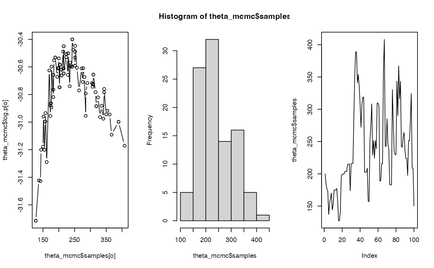
# iv) Visualise samples (log-likelihoods, histogram, MCMC chain)
# > Note the noise in the log-likelihoods due to the stochastic nature of the filter
pp <- par(mfrow = c(1, 3))
o <- order(theta_mcmc$samples)
plot(theta_mcmc$samples[o], theta_mcmc$log.p[o], type = "b")
hist(theta_mcmc$samples)
plot(theta_mcmc$samples, type = "l")
par(pp)
}
}
#> `patter::julia_connect()` called @ 2025-04-22 09:31:02...
#> ... Running `Julia` setup via `JuliaCall::julia_setup()`...
#> ... Validating Julia installation...
#> ... Setting up Julia project...
#> ... Handling dependencies...
#> ... `Julia` set up with 11 thread(s).
#> `patter::julia_connect()` call ended @ 2025-04-22 09:31:02 (duration: ~0 sec(s)).


 #> `patter::pf_filter()` called @ 2025-04-22 09:31:02...
#> `patter::pf_filter_init()` called @ 2025-04-22 09:31:02...
#> ... 09:31:02: Setting initial states...
#> ... 09:31:03: Setting observations dictionary...
#> `patter::pf_filter_init()` call ended @ 2025-04-22 09:31:03 (duration: ~1 sec(s)).
#> ... 09:31:03: Running filter...
#> Message: On iteration 1 ...
#>
#> Message: Running filter for batch 1 / 1 ...
#>
#> ... 09:31:04: Collating outputs...
#> `patter::pf_filter()` call ended @ 2025-04-22 09:31:04 (duration: ~2 sec(s)).
#> `patter::pf_filter()` called @ 2025-04-22 09:31:02...
#> `patter::pf_filter_init()` called @ 2025-04-22 09:31:02...
#> ... 09:31:02: Setting initial states...
#> ... 09:31:03: Setting observations dictionary...
#> `patter::pf_filter_init()` call ended @ 2025-04-22 09:31:03 (duration: ~1 sec(s)).
#> ... 09:31:03: Running filter...
#> Message: On iteration 1 ...
#>
#> Message: Running filter for batch 1 / 1 ...
#>
#> ... 09:31:04: Collating outputs...
#> `patter::pf_filter()` call ended @ 2025-04-22 09:31:04 (duration: ~2 sec(s)).
 #> `patter::map_dens()` called @ 2025-04-22 09:31:04...
#> ... 09:31:04: Processing `.map`...
#> ... 09:31:04: Building XYM...
#> ... 09:31:04: Defining `ppp` object...
#> Observation window is gridded.
#> ... 09:31:04: Estimating density surface...
#> ... 09:31:04: Scaling density surface...
#> `patter::map_dens()` called @ 2025-04-22 09:31:04...
#> ... 09:31:04: Processing `.map`...
#> ... 09:31:04: Building XYM...
#> ... 09:31:04: Defining `ppp` object...
#> Observation window is gridded.
#> ... 09:31:04: Estimating density surface...
#> ... 09:31:04: Scaling density surface...
 #> `patter::map_dens()` call ended @ 2025-04-22 09:31:05 (duration: ~1 sec(s)).

 #> `patter::pf_filter()` called @ 2025-04-22 09:31:05...
#> `patter::pf_filter_init()` called @ 2025-04-22 09:31:05...
#> ... 09:31:05: Setting initial states...
#> ... 09:31:05: Setting observations dictionary...
#> `patter::pf_filter_init()` call ended @ 2025-04-22 09:31:05 (duration: ~0 sec(s)).
#> ... 09:31:05: Running filter...
#> Message: On iteration 1 ...
#>
#> Message: Running filter for batch 1 / 1 ...
#>
#> ... 09:31:05: Collating outputs...
#> `patter::pf_filter()` call ended @ 2025-04-22 09:31:05 (duration: ~0 sec(s)).
#> `patter::pf_filter()` called @ 2025-04-22 09:31:05...
#> `patter::pf_filter_init()` called @ 2025-04-22 09:31:05...
#> ... 09:31:05: Setting initial states...
#> ... 09:31:05: Setting observations dictionary...
#> `patter::pf_filter_init()` call ended @ 2025-04-22 09:31:05 (duration: ~0 sec(s)).
#> ... 09:31:05: Running filter...
#> Message: On iteration 1 ...
#>
#> Message: Running filter for batch 1 / 1 ...
#>
#> ... 09:31:06: Collating outputs...
#> `patter::pf_filter()` call ended @ 2025-04-22 09:31:06 (duration: ~1 sec(s)).
#> `patter::pf_filter()` called @ 2025-04-22 09:31:06...
#> `patter::pf_filter_init()` called @ 2025-04-22 09:31:06...
#> ... 09:31:06: Setting initial states...
#> ... 09:31:06: Setting observations dictionary...
#> `patter::pf_filter_init()` call ended @ 2025-04-22 09:31:06 (duration: ~0 sec(s)).
#> ... 09:31:06: Running filter...
#> Message: On iteration 1 ...
#>
#> Message: Running filter for batch 1 / 1 ...
#>
#> ... 09:31:06: Collating outputs...
#> `patter::pf_filter()` call ended @ 2025-04-22 09:31:06 (duration: ~0 sec(s)).
#> `patter::pf_filter()` called @ 2025-04-22 09:31:06...
#> `patter::pf_filter_init()` called @ 2025-04-22 09:31:06...
#> ... 09:31:06: Setting initial states...
#> ... 09:31:06: Setting observations dictionary...
#> `patter::pf_filter_init()` call ended @ 2025-04-22 09:31:06 (duration: ~0 sec(s)).
#> ... 09:31:06: Running filter...
#> Message: On iteration 1 ...
#>
#> Message: Running filter for batch 1 / 1 ...
#>
#> ... 09:31:07: Collating outputs...
#> `patter::pf_filter()` call ended @ 2025-04-22 09:31:07 (duration: ~1 sec(s)).
#> `patter::pf_filter()` called @ 2025-04-22 09:31:07...
#> `patter::pf_filter_init()` called @ 2025-04-22 09:31:07...
#> ... 09:31:07: Setting initial states...
#> ... 09:31:07: Setting observations dictionary...
#> `patter::pf_filter_init()` call ended @ 2025-04-22 09:31:07 (duration: ~0 sec(s)).
#> ... 09:31:07: Running filter...
#> Message: On iteration 1 ...
#>
#> Message: Running filter for batch 1 / 1 ...
#>
#> ... 09:31:07: Collating outputs...
#> `patter::pf_filter()` call ended @ 2025-04-22 09:31:07 (duration: ~0 sec(s)).
#> `patter::pf_filter()` called @ 2025-04-22 09:31:05...
#> `patter::pf_filter_init()` called @ 2025-04-22 09:31:05...
#> ... 09:31:05: Setting initial states...
#> ... 09:31:05: Setting observations dictionary...
#> `patter::pf_filter_init()` call ended @ 2025-04-22 09:31:05 (duration: ~0 sec(s)).
#> ... 09:31:05: Running filter...
#> Message: On iteration 1 ...
#>
#> Message: Running filter for batch 1 / 1 ...
#>
#> ... 09:31:05: Collating outputs...
#> `patter::pf_filter()` call ended @ 2025-04-22 09:31:05 (duration: ~0 sec(s)).
#> `patter::pf_filter()` called @ 2025-04-22 09:31:05...
#> `patter::pf_filter_init()` called @ 2025-04-22 09:31:05...
#> ... 09:31:05: Setting initial states...
#> ... 09:31:05: Setting observations dictionary...
#> `patter::pf_filter_init()` call ended @ 2025-04-22 09:31:05 (duration: ~0 sec(s)).
#> ... 09:31:05: Running filter...
#> Message: On iteration 1 ...
#>
#> Message: Running filter for batch 1 / 1 ...
#>
#> ... 09:31:06: Collating outputs...
#> `patter::pf_filter()` call ended @ 2025-04-22 09:31:06 (duration: ~1 sec(s)).
#> `patter::pf_filter()` called @ 2025-04-22 09:31:06...
#> `patter::pf_filter_init()` called @ 2025-04-22 09:31:06...
#> ... 09:31:06: Setting initial states...
#> ... 09:31:06: Setting observations dictionary...
#> `patter::pf_filter_init()` call ended @ 2025-04-22 09:31:06 (duration: ~0 sec(s)).
#> ... 09:31:06: Running filter...
#> Message: On iteration 1 ...
#>
#> Message: Running filter for batch 1 / 1 ...
#>
#> ... 09:31:06: Collating outputs...
#> `patter::pf_filter()` call ended @ 2025-04-22 09:31:06 (duration: ~0 sec(s)).
#> `patter::pf_filter()` called @ 2025-04-22 09:31:06...
#> `patter::pf_filter_init()` called @ 2025-04-22 09:31:06...
#> ... 09:31:06: Setting initial states...
#> ... 09:31:06: Setting observations dictionary...
#> `patter::pf_filter_init()` call ended @ 2025-04-22 09:31:06 (duration: ~0 sec(s)).
#> ... 09:31:06: Running filter...
#> Message: On iteration 1 ...
#>
#> Message: Running filter for batch 1 / 1 ...
#>
#> ... 09:31:07: Collating outputs...
#> `patter::pf_filter()` call ended @ 2025-04-22 09:31:07 (duration: ~1 sec(s)).
#> `patter::pf_filter()` called @ 2025-04-22 09:31:07...
#> `patter::pf_filter_init()` called @ 2025-04-22 09:31:07...
#> ... 09:31:07: Setting initial states...
#> ... 09:31:07: Setting observations dictionary...
#> `patter::pf_filter_init()` call ended @ 2025-04-22 09:31:07 (duration: ~0 sec(s)).
#> ... 09:31:07: Running filter...
#> Message: On iteration 1 ...
#>
#> Message: Running filter for batch 1 / 1 ...
#>
#> ... 09:31:07: Collating outputs...
#> `patter::pf_filter()` call ended @ 2025-04-22 09:31:07 (duration: ~0 sec(s)).
#> `patter::pf_filter()` called @ 2025-04-22 09:31:07...
#> `patter::pf_filter_init()` called @ 2025-04-22 09:31:07...
#> ... 09:31:07: Setting initial states...
#> ... 09:31:07: Setting observations dictionary...
#> `patter::pf_filter_init()` call ended @ 2025-04-22 09:31:07 (duration: ~0 sec(s)).
#> ... 09:31:07: Running filter...
#> Message: On iteration 1 ...
#>
#> Message: Running filter for batch 1 / 1 ...
#>
#> ... 09:31:07: Collating outputs...
#> `patter::pf_filter()` call ended @ 2025-04-22 09:31:07 (duration: ~0 sec(s)).
 #> `patter::pf_filter()` called @ 2025-04-22 09:31:08...
#> `patter::pf_filter_init()` called @ 2025-04-22 09:31:08...
#> ... 09:31:08: Setting initial states...
#> ... 09:31:08: Setting observations dictionary...
#> `patter::pf_filter_init()` call ended @ 2025-04-22 09:31:08 (duration: ~0 sec(s)).
#> ... 09:31:08: Running filter...
#> Message: On iteration 1 ...
#>
#> Message: Running filter for batch 1 / 1 ...
#>
#> ... 09:31:09: Collating outputs...
#> `patter::pf_filter()` call ended @ 2025-04-22 09:31:09 (duration: ~1 sec(s)).
#> `patter::pf_filter()` called @ 2025-04-22 09:31:09...
#> `patter::pf_filter_init()` called @ 2025-04-22 09:31:09...
#> ... 09:31:09: Setting initial states...
#> ... 09:31:09: Setting observations dictionary...
#> `patter::pf_filter_init()` call ended @ 2025-04-22 09:31:09 (duration: ~0 sec(s)).
#> ... 09:31:09: Running filter...
#> Message: On iteration 1 ...
#>
#> Message: Running filter for batch 1 / 1 ...
#>
#> ... 09:31:09: Collating outputs...
#> `patter::pf_filter()` call ended @ 2025-04-22 09:31:10 (duration: ~1 sec(s)).
#> `patter::pf_filter()` called @ 2025-04-22 09:31:08...
#> `patter::pf_filter_init()` called @ 2025-04-22 09:31:08...
#> ... 09:31:08: Setting initial states...
#> ... 09:31:08: Setting observations dictionary...
#> `patter::pf_filter_init()` call ended @ 2025-04-22 09:31:08 (duration: ~0 sec(s)).
#> ... 09:31:08: Running filter...
#> Message: On iteration 1 ...
#>
#> Message: Running filter for batch 1 / 1 ...
#>
#> ... 09:31:09: Collating outputs...
#> `patter::pf_filter()` call ended @ 2025-04-22 09:31:09 (duration: ~1 sec(s)).
#> `patter::pf_filter()` called @ 2025-04-22 09:31:09...
#> `patter::pf_filter_init()` called @ 2025-04-22 09:31:09...
#> ... 09:31:09: Setting initial states...
#> ... 09:31:09: Setting observations dictionary...
#> `patter::pf_filter_init()` call ended @ 2025-04-22 09:31:09 (duration: ~0 sec(s)).
#> ... 09:31:09: Running filter...
#> Message: On iteration 1 ...
#>
#> Message: Running filter for batch 1 / 1 ...
#>
#> ... 09:31:09: Collating outputs...
#> `patter::pf_filter()` call ended @ 2025-04-22 09:31:10 (duration: ~1 sec(s)).


 #> generate 100 samples