Map: probability-of-use

This function builds a 'probability-of-use' utilisation distribution.

Usage

map_pou(
  .map,
  .coord,
  .plot = TRUE,
  ...,
  .verbose = getOption("patter.verbose")
)

Arguments

.map

A terra::SpatRaster that defines the grid for probability-of-use estimation.

.coord

Coordinates, provided in any format accepted by .map_coord()

.plot, ...

A logical input that defines whether or not to plot the terra::SpatRaster and additional arguments passed to terra::plot().

.verbose

User output control (see patter-progress for supported options).

Value

The function returns a named list with the following elements:

• ud: a normalised terra::SpatRaster;

Details

Probability-of-use is calculated via .map_coord() (and .map_mark()). If a single dataset of unweighted coordinates is provided, probability-of-use is simply the proportion of records in each grid cell. If a time series of unweighted coordinates is provided, probability-of-use is effectively the average proportion of records in each grid cell. This becomes a weighted average if coordinates are weighted. Weights are normalised to sum to one and the result can be interpreted as a utilisation distribution in which cell values define probability-of-use. Maps are sensitive to grid resolution.

This function replaces flapper::pf_plot_map().

On Linux, this function cannot be used within a Julia session.

See also

map_*() functions build maps of space use:

• map_pou() maps probability-of-use;

• map_dens() maps point density;

• map_hr_*() functions map home ranges;

All maps are represented as terra::SpatRasters.

To derive coordinates for mapping patterns of space use for tagged animals, see:

• coa() to calculate centre-of-activity;

• pf_filter() and associates to sample locations using particle filtering;

Author

Edward Lavender

Examples

if (patter_run(.julia = FALSE, .geospatial = TRUE)) {

  library(data.table)
  library(dtplyr)
  library(dplyr, warn.conflicts = FALSE)

  #### Define map
  map <- dat_gebco()

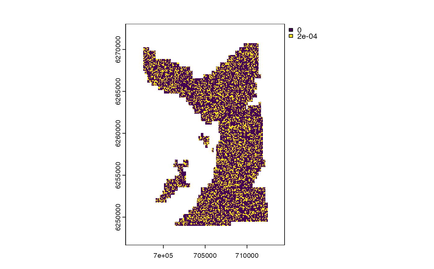
  #### Example (1): Use sample coordinates
  # Sample example coordinates
  coord <-
    map |>
    terra::spatSample(size = 5000L, xy = TRUE, cell = TRUE, na.rm = TRUE) |>
    select("x", "y") |>
    as.data.table()
  # Use x, y coordinates
  map_pou(map, .coord = coord)
  # Other formats are acceptable
  map_pou(map, .coord = as.matrix(coord))
  map_pou(map, .coord = as.data.frame(coord))
  # `cell_x` and `cell_y` coordinates are acceptable
  map_pou(map, .coord = coord[, .(cell_x = x, cell_y = y)])

  #### Example (2): Use coordinates from `coa()`
  # Use example dataset
  coord <- dat_coa()
  map_pou(map, .coord = coord)
  points(coord$x, coord$y, cex = 0.5)

  #### Example (3): Use a time series of coordinates from `pf_*()`
  # Use example dataset
  # * We use particles from the forward filter (`?pf_filter()`);
  # * Particles are equally weighted b/c re-sampling is implemented every time step;
  # * It is better to use outputs from the particle smoother;
  coord <- dat_pff()$states
  map_pou(map, .coord = coord)
  # points(coord$x, coord$y, cex = 0.5)

}
#> `patter::map_pou()` called @ 2025-04-22 09:31:00... 
#> ... Building XYM... 
#> ... Building SpatRaster... 

#> `patter::map_pou()` call ended @ 2025-04-22 09:31:00 (duration: ~0 sec(s)). 
#> `patter::map_pou()` called @ 2025-04-22 09:31:00... 
#> ... Building XYM... 
#> ... Building SpatRaster... 
#> `patter::map_pou()` call ended @ 2025-04-22 09:31:00 (duration: ~0 sec(s)). 
#> `patter::map_pou()` called @ 2025-04-22 09:31:00... 
#> ... Building XYM... 
#> ... Building SpatRaster... 
#> `patter::map_pou()` call ended @ 2025-04-22 09:31:00 (duration: ~0 sec(s)). 
#> `patter::map_pou()` called @ 2025-04-22 09:31:00... 
#> ... Building XYM... 
#> ... Building SpatRaster... 
#> `patter::map_pou()` call ended @ 2025-04-22 09:31:00 (duration: ~0 sec(s)). 
#> `patter::map_pou()` called @ 2025-04-22 09:31:00... 
#> ... Building XYM... 
#> ... Building SpatRaster... 

#> `patter::map_pou()` call ended @ 2025-04-22 09:31:00 (duration: ~0 sec(s)). 
#> `patter::map_pou()` called @ 2025-04-22 09:31:00... 
#> ... Building XYM... 
#> ... Building SpatRaster... 

#> `patter::map_pou()` call ended @ 2025-04-22 09:31:00 (duration: ~0 sec(s)). 
#> $ud
#> class       : SpatRaster 
#> dimensions  : 264, 190, 1  (nrow, ncol, nlyr)
#> resolution  : 100, 100  (x, y)
#> extent      : 695492.1, 714492.1, 6246657, 6273057  (xmin, xmax, ymin, ymax)
#> coord. ref. : WGS 84 / UTM zone 29N (EPSG:32629) 
#> source(s)   : memory
#> varname     : dat_gebco 
#> name        :   map_value 
#> min value   : 0.000000000 
#> max value   : 0.003333333 
#>