COA: centres of activity

This function calculates centres of activity (COAs) from detections at acoustic receivers.

Usage

coa(
  .map,
  .detections,
  .moorings = NULL,
  .delta_t,
  .split = NULL,
  .plot_weights = TRUE,
  ...,
  .one_page = TRUE
)

Arguments

.map

A terra::SpatRaster that defines the study area (see glossary). Here, .map is used to:

• Extract map_value at centres of activity, for consistency with other routines (such as pf_filter());

.detections, .moorings

Acoustic detection data.table::data.table.

• .detections is a data.table::data.table of acoustic detections, with the following columns: receiver_id (or sensor_id), timestamp and (optionally) receiver_x and receiver_y columns;

• (optional) .moorings is a data.table::data.table of receiver coordinates, which should be provided if unavailable in .detections, with receiver_id, receiver_x and receiver_y columns;

Receiver coordinates must be planar.

.delta_t

The time interval over which to calculate COAs. This can be specified in any way understood by lubridate::floor_date() (see the unit argument).

.split

(optional) A character that defines the name of the grouping factor in .detections (e.g., individual_id for dat_detections).

.plot_weights, ..., .one_page

Plot arguments.

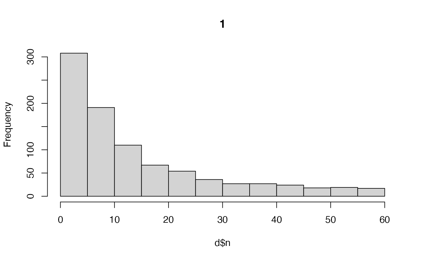
• .plot_weights is a logical variable that defines whether or not to plot the frequency distribution of weights for each .split value (i.e., the frequency distribution of the number of detections at each receiver in each time interval, excluding time intervals without detections).

• ... is a placeholder for arguments passed to graphics::hist(), excluding main.

• .one_page A logical variable that defines whether or not to plot all histograms on one page.

Value

The function returns a data.table::data.table with the following columns:

• {.split}—a character vector that distinguishes groups, if applicable;

• timestep—an integer vector of time steps;

• timestamp—a POSIXt vector of time stamps;

• map_value, x, y—the value of .map at COAs and their coordinates;

Data are arranged by .split and timestamp.

Details

COAs are calculated as a weighted mean of the locations of receivers at which individuals are detected over consecutive time intervals, weighted by the frequency of detections at each of those receivers. COAs are calculated via stats::weighted.mean(), which assumes planar coordinates, for consistency with other patter routines. To handle longitude/latitude coordinates, use geosphere::geomean().

This function replaces flapper::coa(). See flapper::coa_setup_delta_t() to evaluate alternative time internals.

On Linux, this function cannot be used within a Julia session.

See also

• To derive location samples from a particle filtering algorithm, see pf_filter() and associates;

• For mapping utilisation distributions from coordinates, see map_*() functions (i.e., map_pou() and map_dens());

Author

Edward Lavender

Examples

if (patter_run(.julia = FALSE, .geospatial = TRUE)) {

  library(data.table)

  #### Set up example
  map        <- dat_gebco()
  detections <- dat_detections
  moorings   <- dat_moorings

  #### Example (1): Calculate COAs for an example individual
  id     <- dat_detections$individual_id[1]
  det    <- dat_detections[individual_id == id, ]
  coa(.map = map, .detections = det, .moorings = moorings,
      .delta_t = "2 hours")

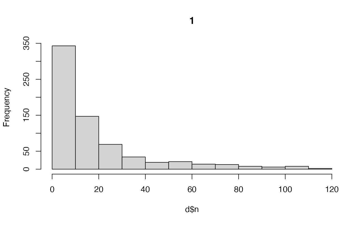
  #### Example (2): Customise the time interval via `.delta_t`
  coa(.map = map, .detections = det, .moorings = moorings,
      .delta_t = "4 hours")

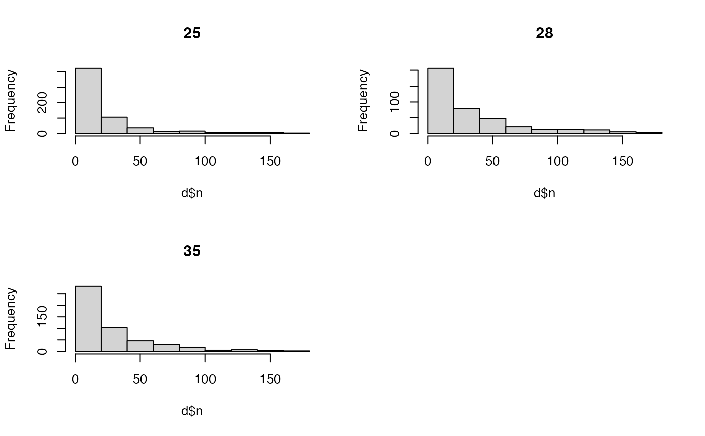
  #### Example (3): Calculate COAs for multiple individuals via `.split`
  # Calculate COAs
  coa(.map = map, .detections = det, .moorings = moorings,
      .delta_t = "6 hours", .split = "individual_id")
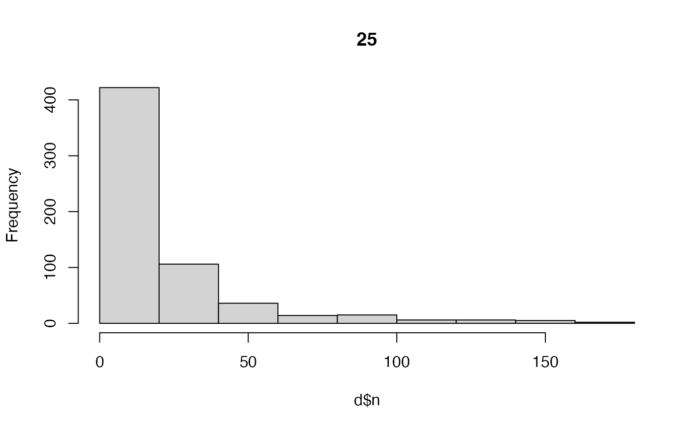
  # Use one page for plots via `.one_page = TRUE`
  coa(.map = map, .detections = det, .moorings = moorings,
      .delta_t = "6 hours", .split = "individual_id",
      .one_page = FALSE)
  # Suppress plots via `.plot = FALSE`
  coa(.map = map, .detections = det, .moorings = moorings,
      .delta_t = "6 hours", .split = "individual_id",
      .one_page = TRUE)

  #### Example (4): Specify `.detections` only
  # `.moorings` is not required if `.detections` contains receiver coordinates
  coa(.map = map,
      .detections =
        detections |>
        merge(moorings, by = "receiver_id"),
      .delta_t = "6 hours", .split = "individual_id")

}






#>       individual_id timestep           timestamp map_value        x       y
#>               <int>    <int>              <POSc>     <num>    <num>   <num>
#>    1:            25        1 2016-03-17 00:00:00  59.76520 709120.1 6253030
#>    2:            25        2 2016-03-17 06:00:00  49.72233 709398.4 6253169
#>    3:            25        3 2016-03-21 18:00:00  58.17422 709242.1 6253107
#>    4:            25        4 2016-03-22 00:00:00  58.17422 709242.1 6253107
#>    5:            25        5 2016-03-22 06:00:00  58.17422 709242.1 6253107
#>   ---                                                                      
#> 1204:            35      402 2017-04-10 18:00:00  99.90396 709048.8 6253427
#> 1205:            35      403 2017-04-11 18:00:00  49.51562 706342.1 6254307
#> 1206:            35      404 2017-04-12 00:00:00 117.36553 707042.1 6253840
#> 1207:            35      405 2017-04-12 18:00:00 113.60658 708771.2 6253210
#> 1208:            35      406 2017-04-19 18:00:00 129.77667 707242.1 6253707