Simulation: movement walks

Simulate discrete-time animal movement paths from walk models (e.g., random walks, biased random walks, correlated random walks).

sim_path_walk(
  .map,
  .timeline,
  .state = "StateXY",
  .xinit = NULL,
  .n_path = 1L,
  .model_move = move_xy(),
  .plot = TRUE,
  .one_page = FALSE
)

Arguments

.map

A SpatRaster that defines the study area for the simulation (see glossary). Here, .map is used to:

• Simulate initial states if .xinit = NULL (via sim_states_init());

.timeline

A POSIXct vector of regularly spaced time stamps that defines the timeline for the simulation. Here, .timeline is used to:

• Define the number of time steps for the simulation;

• Define the time resolution of the simulation;

.state

A character that defines the State type (see glossary).

.xinit, .n_path

Initial State arguments.

• .xinit specifies the initial states for the simulation (one for each movement path).

  • If .xinit is NULL, initial states are sampled from .map (via sim_states_init()).

  • Otherwise, .xinit must be a data.table with one column for each state dimension.

• .n_path is an integer that defines the number of paths to simulate.

.model_move

A character string that defines the movement model (see ModelMove and glossary).

.plot, .one_page

Plot options.

• .plot is a logical variable that defined whether or not to plot .map and simulated path(s). Each path is plotted on a separate plot.

• .one_page is a logical variable that defines whether or not to produce all plots on a single page.

Value

sim_path_walk() returns a data.table with the following columns:

• path_id---an integer vector that identifies each path;

• timestep---an integer vector that defines the time step;

• timestamp---a POSIXct vector of time stamps;

• x,y,...---numeric vectors that define the components of the state;

Details

This function simulates movement paths via Patter.simulate_path_walk():

• The internal function sim_states_init() is used to set the initial state(s) for the simulation; that is, initial coordinates and other variables (one for each .n_path). If .state is one of the built-in options (see State), initial state(s) can be sampled from .map. Otherwise, additional methods or a data.table of initial states must be provided (see sim_states_init()). Initial states provided in .xinit are re-sampled, with replacement, if required, such that there is one initial state for each simulated path. Initial states are assigned to an xinit object in Julia, which is a Vector of States.

• Using the initial states, the Julia function Patter.simulate_path_walk() simulates movement path(s) using the movement model (.model_move).

• Movement paths are passed back to R for convenient visualisation and analysis.

To use a new .state and/or .model_move sub-type for sim_path_walk():

• Define a State sub-type in Julia and provide the name as a character string to this function;

• To initialise the simulation, write a states_init() method to enable automated sampling of initial states via sim_states_init() or provide a data.table of initial states to .xinit;

• Define a corresponding ModelMove sub-type in Julia;

• Instantiate a ModelMove instance (that is, define a specific movement model);

sim_path_walk() replaces flapper::sim_path_sa(). Other flapper::sim_path_*() functions are not currently implemented in patter.

See also

• sim_* functions implement de novo simulation of movements and observations:

  • sim_path_walk() simulates movement path(s) (via ModelMove);

  • sim_array() simulates acoustic array(s);

  • sim_observations() simulates observations (via ModelObs);

Author

Edward Lavender

Examples

if (julia_run()) {

  library(data.table)
  library(dtplyr)
  library(dplyr, warn.conflicts = FALSE)

  #### Connect to Julia
  julia_connect()
  set_seed()

  #### Set up study system
  # Define `map` (the region within which movements are permitted)
  map <- dat_gebco()
  set_map(map)
  # Define study period
  timeline <- seq(as.POSIXct("2016-01-01", tz = "UTC"),
                  length.out = 1000L, by = "2 mins")

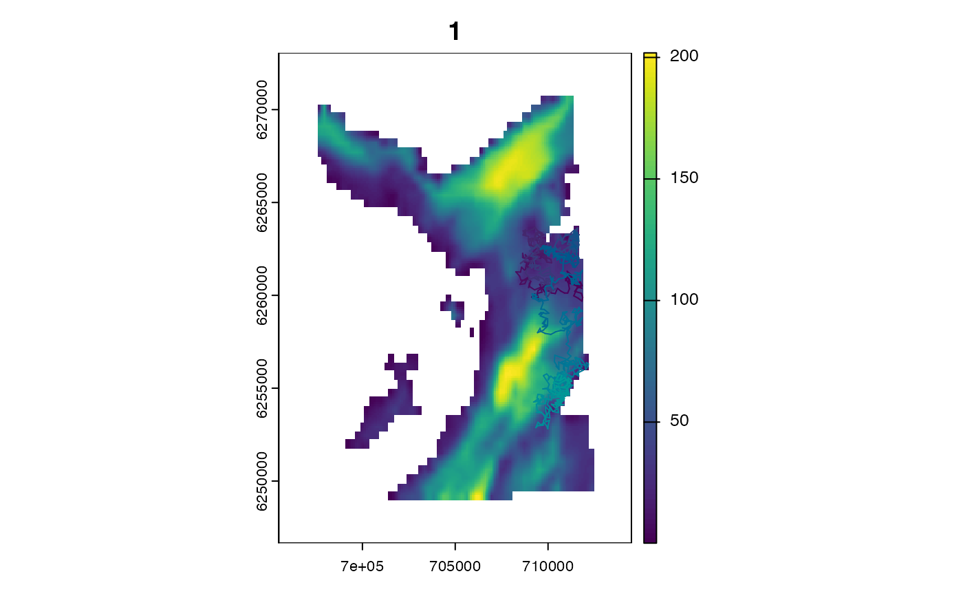
  #### Example (1): Simulate path with default options
  sim_path_walk(.map = map,
                .timeline = timeline,
                .state = "StateXY",
                .model_move = move_xy())

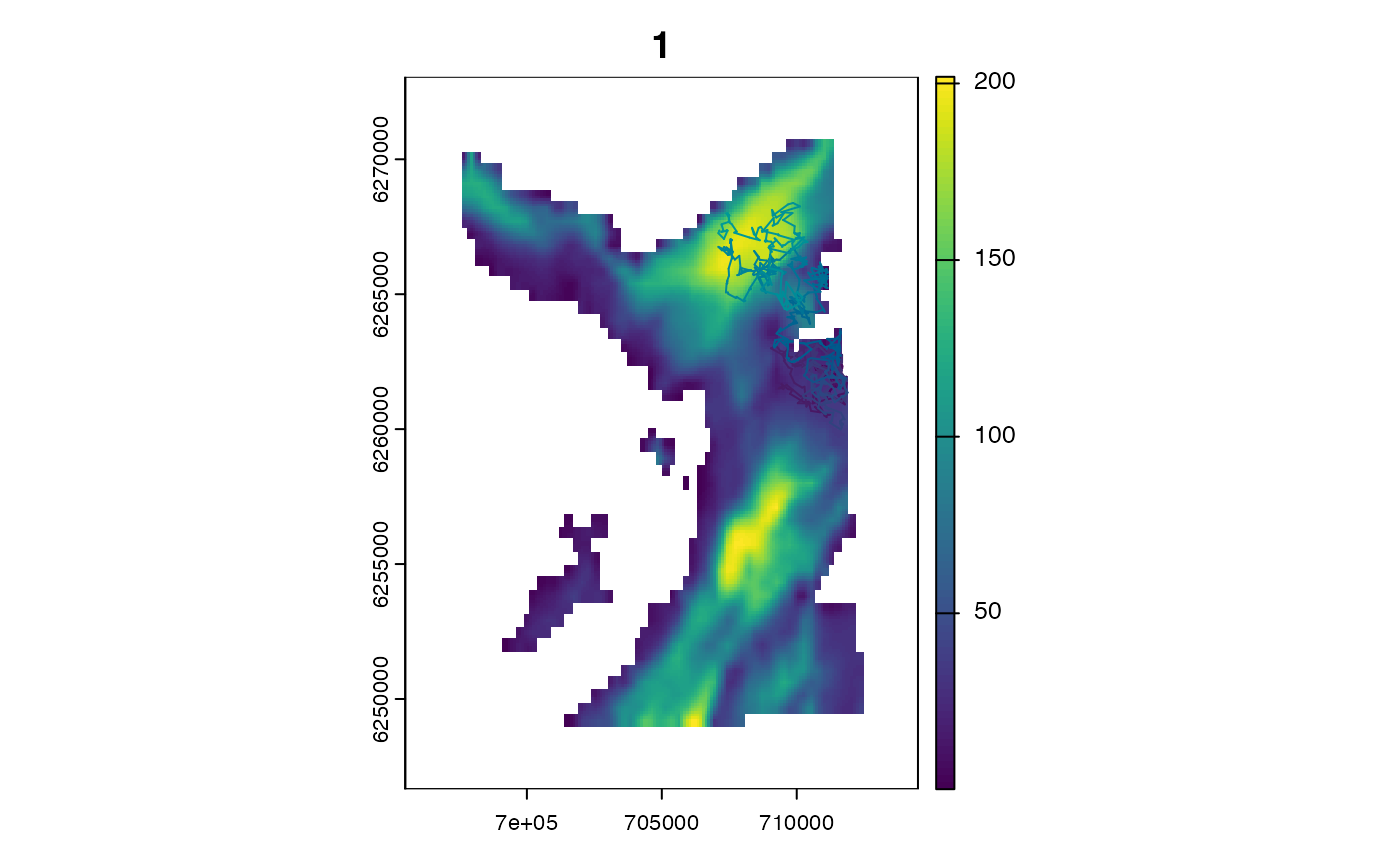
  #### Example (2): Set the starting location via `.xinit`
  # Define an initial location
  x <- 708212.6
  y <- 6251684
  origin <- data.table(map_value = terra::extract(map, cbind(x, y))[1, 1],
                       x = x, y = y)
  # Run the simulation
  sim_path_walk(.map = map,
                .timeline = timeline,
                .state = "StateXY",
                .xinit = origin,
                .model_move = move_xy())
  points(origin$x, origin$y)

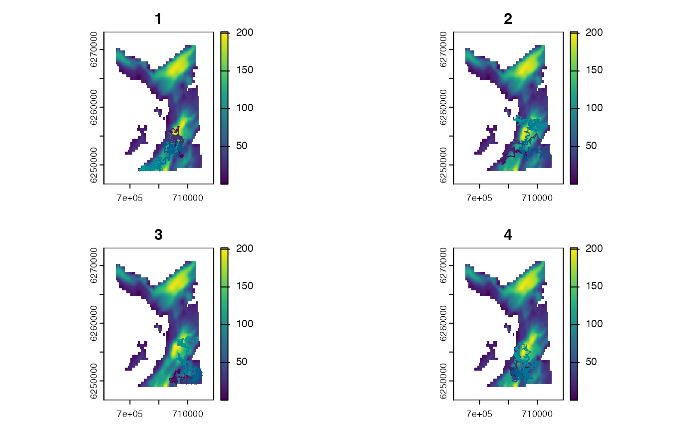
  #### Example (3): Simulate multiple paths with the same origin via `.xinit`
  sim_path_walk(.map = map,
                .timeline = timeline,
                .state = "StateXY",
                .xinit = origin,
                .model_move = move_xy(),
                .n_path = 4L,
                .one_page = TRUE)

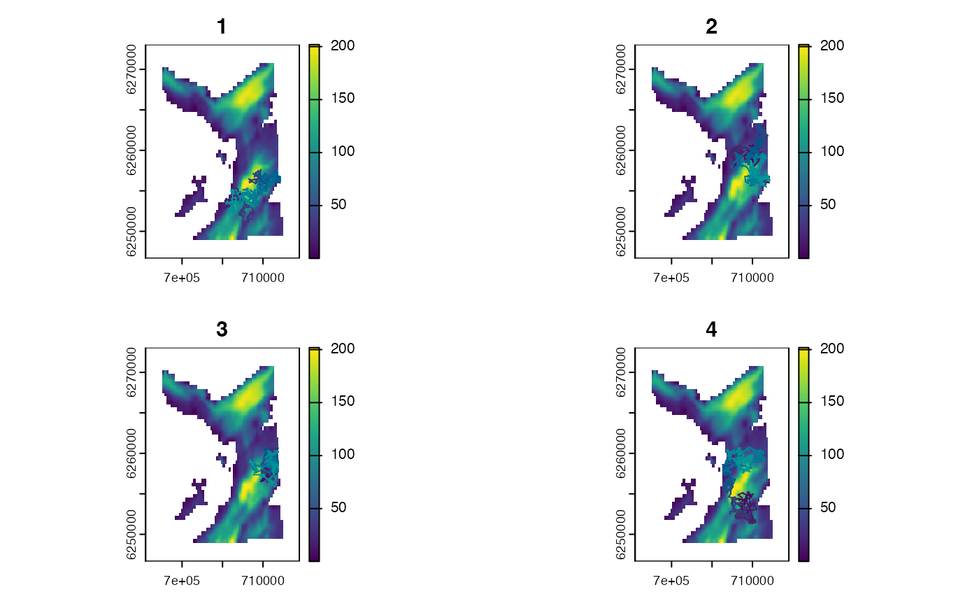
  #### Example (4): Simulate multiple paths with different origins via `.xinit`
  # Manually specify origins
  origins <-
    map |>
    terra::spatSample(size = 4, xy = TRUE, na.rm = TRUE) |>
    select("map_value", "x", "y") |>
    as.data.table()
  # Run simulation
  sim_path_walk(.map = map,
                .timeline = timeline,
                .state = "StateXY",
                .xinit = origins,
                .model_move = move_xy(),
                .n_path = 4L,
                .one_page = TRUE)

  #### Example (5): Customise two-dimensional random walks via `move_xy()`
  # Adjust distributions for step lengths and turning angles
  move <- move_xy(dbn_length = "truncated(Normal(250, 50), lower = 0.0, upper = 750.0)",
                  dbn_angle = "VonMises(0.1, 0.1)")
  sim_path_walk(.map = map,
                .timeline = timeline,
                .state = "StateXY",
                .model_move = move)
  # Experiment with other options
  move <- move_xy(dbn_length = "truncated(Normal(10, 50), lower = 0.0, upper = 300)")
  sim_path_walk(.map = map,
                .timeline = timeline,
                .state = "StateXY",
                .model_move = move)

  #### Example (6): Use other .state/.model_move combinations
  # Simulate a correlated random walk
  sim_path_walk(.map = map,
                .timeline = timeline,
                .state = "StateXYZD",
                .model_move = move_xyzd())
  # Modify movement model parameters
  sim_path_walk(.map = map,
                .timeline = timeline,
                .state = "StateXYZD",
                .model_move = move_xyzd(dbn_angle_delta = "Normal(0, 1)",
                                        dbn_z_delta = "Normal(0, 0.5)"))

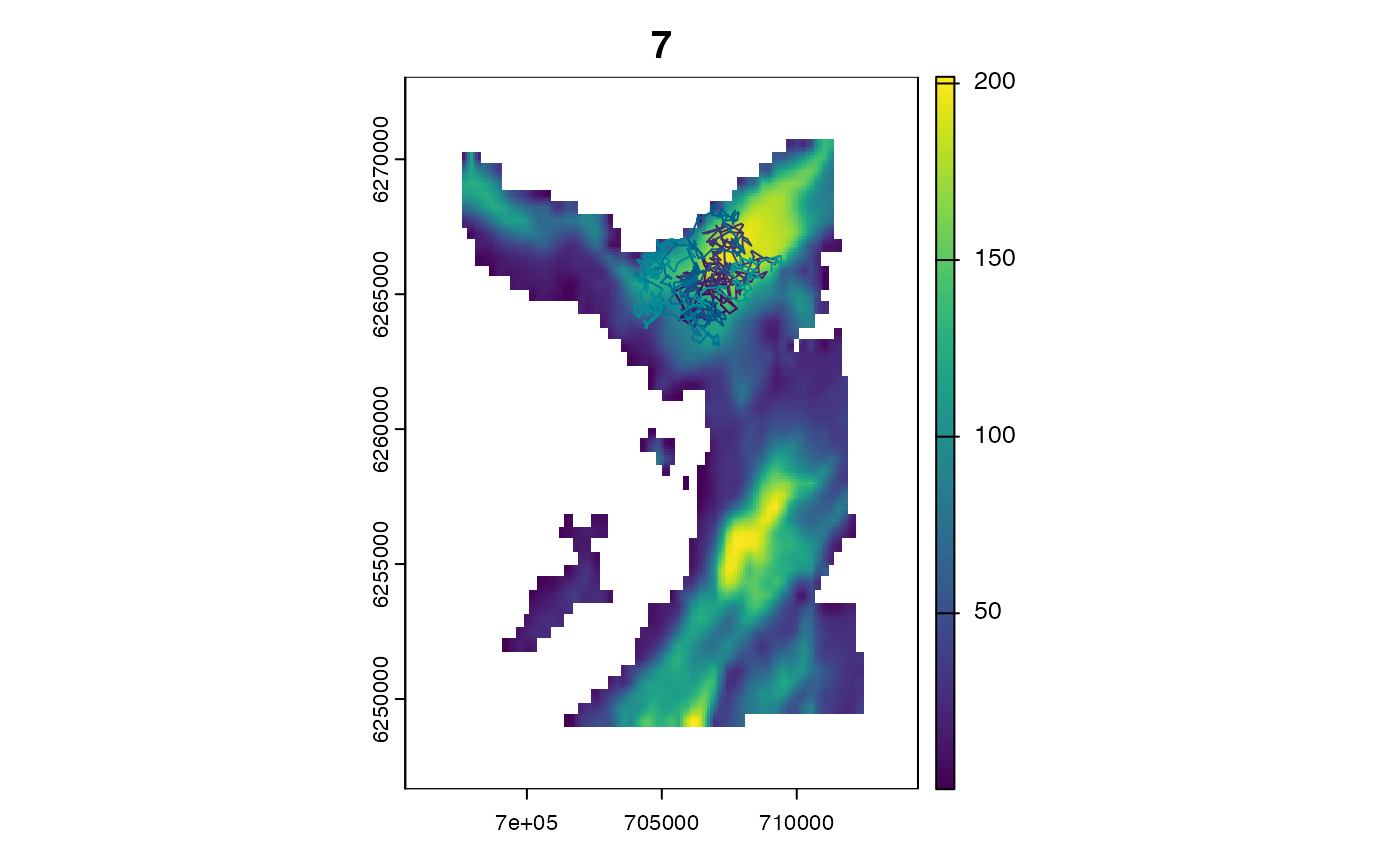
  #### Example (7): Use custom .state/.model_move sub-types
  # See `?State` and ?ModelMove`

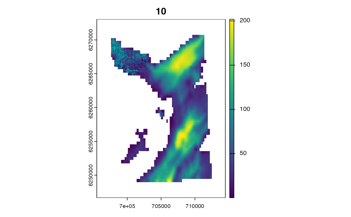
  #### Example (8): Simulate numerous paths via `.n_path`
  sim_path_walk(.map = map,
                .timeline = timeline,
                .state = "StateXY",
                .model_move = move_xy(),
                .n_path = 10L)

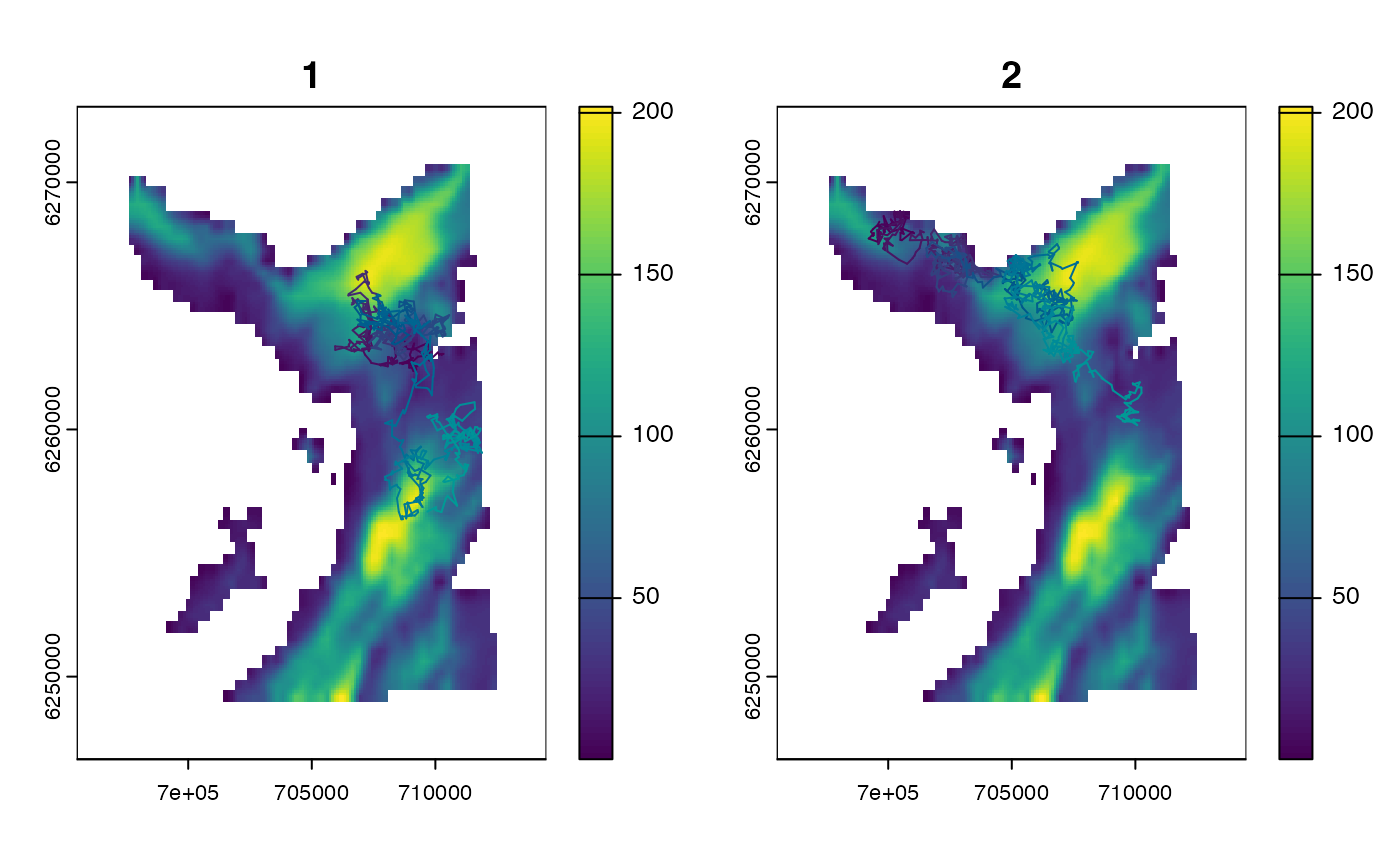
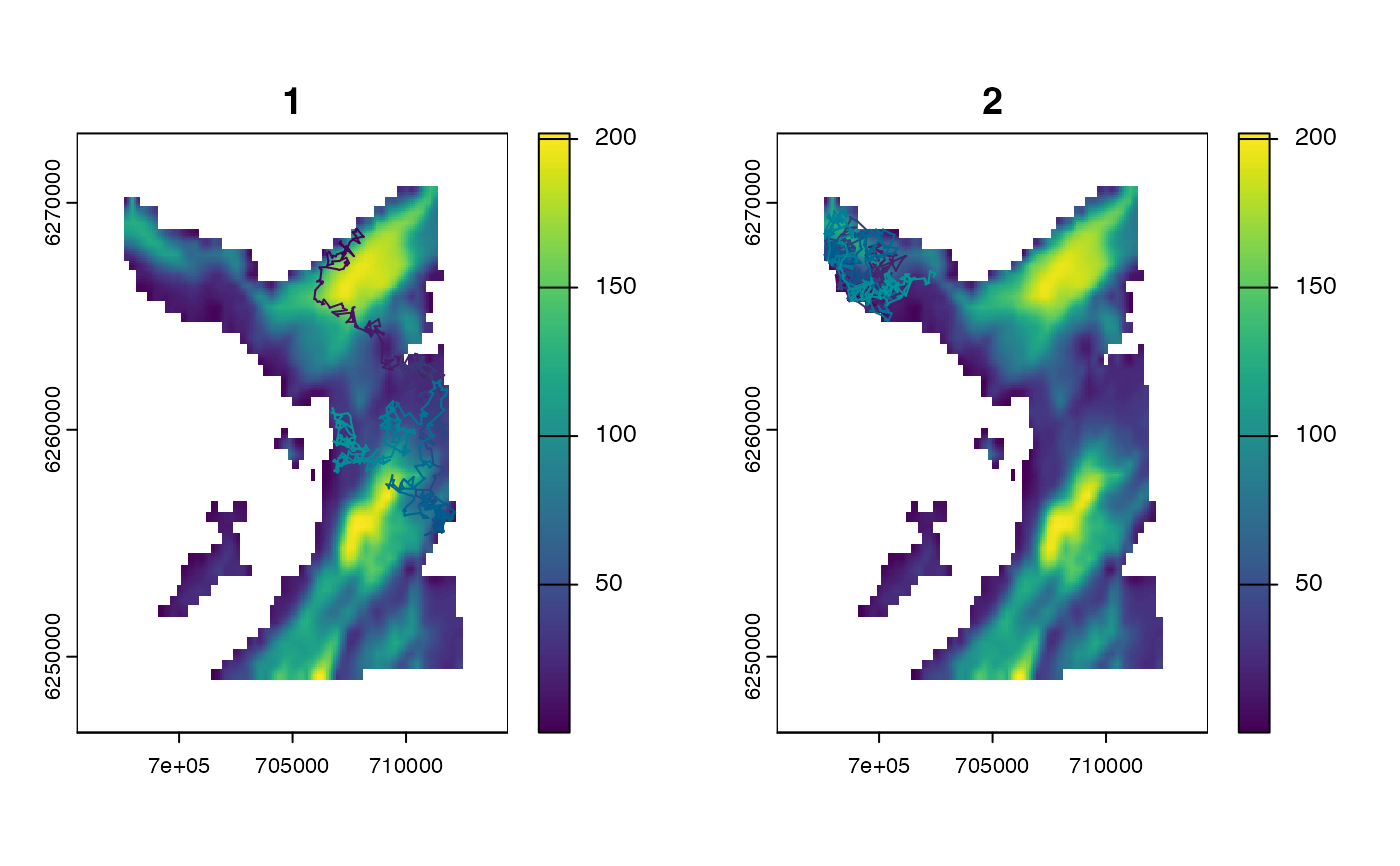
  #### Example (9): Customise plotting options via `.plot` & `.one_page`
  # Use one page via `.one_page = TRUE`
  sim_path_walk(.map = map,
                .timeline = timeline,
                .state = "StateXY",
                .model_move = move_xy(),
                .n_path = 2L, .one_page = TRUE)
  # Suppress plots via `.plot = FALSE`
  sim_path_walk(.map = map,
                .timeline = timeline,
                .state = "StateXY",
                .model_move = move_xy(),
                .plot = FALSE)

}
#> `patter::julia_connect()` called @ 2024-08-01 11:44:00... 
#> ... Running `Julia` setup via `JuliaCall::julia_setup()`... 
#> ... Validating Julia installation... 
#> ... Setting up Julia project... 
#> ... Handling dependencies... 
#> Warning: `JULIA_NUM_THREADS` could not be set via `.threads`.
#> ... `Julia` set up with 8 thread(s). 
#> `patter::julia_connect()` call ended @ 2024-08-01 11:44:06 (duration: ~6 sec(s)). 



















#>       path_id timestep           timestamp map_value        x       y
#>         <int>    <int>              <POSc>     <num>    <num>   <num>
#>    1:       1        1 2016-01-01 00:00:00 27.389563 702242.1 6254207
#>    2:       1        2 2016-01-01 00:02:00 26.590059 702273.8 6254122
#>    3:       1        3 2016-01-01 00:04:00 26.590059 702271.9 6254105
#>    4:       1        4 2016-01-01 00:06:00 24.991056 702238.3 6253924
#>    5:       1        5 2016-01-01 00:08:00 29.677847 702178.5 6254186
#>   ---                                                                
#>  996:       1      996 2016-01-02 09:10:00 14.078653 699601.8 6252064
#>  997:       1      997 2016-01-02 09:12:00 12.087568 699583.2 6252049
#>  998:       1      998 2016-01-02 09:14:00  9.131541 699450.8 6251831
#>  999:       1      999 2016-01-02 09:16:00 14.796794 699653.6 6251902
#> 1000:       1     1000 2016-01-02 09:18:00 11.904321 699524.2 6252218