Simulation: observations

Simulate a time series of observations, such as acoustic detections and depth measurements, arising from simulated animal movement path(s).

Usage

sim_observations(.timeline, .model_obs, .collect = TRUE)

Arguments

.timeline: A POSIXct vector of regularly spaced time stamps that defines the timeline for the simulation. This should match the .timeline used to simulate movement paths (see sim_path_walk()).
.model_obs: A named list of data.table::data.table. Element names should refer to ModelObs structures. Each element should be a data.table::data.table that defines observation model parameters (see glossary).
.collect: A logical variable that defines whether or not to collect outputs from the Julia session in R.

Value

Patter.simulate_yobs() creates a Dict in the Julia session (named yobs).

If .collect = TRUE, sim_observations() collects the outputs in R as a named list, with one element for each sensor type, that is .model_obs element. Each element is a list of data.table::data.tables, one for each simulated path. Each row is a time step. The columns depend on the model type.

Otherwise, invisible(NULL) is returned.

Details

This function wraps Patter.simulate_yobs(). The function iterates over simulated paths defined in the Julia workspace by sim_path_walk(). For each path and time step, the function simulates observation(s). Collectively, .model_obs names and parameter data.table::data.table define the observation models used for the simulation (that is, a Vector of ModelObs instances). In Julia, simulated observations are stored in a hash table (Dict) called yobs, which is translated into a named list that is returned by R.

Author

Edward Lavender

Examples

if (patter_run(.julia = TRUE, .geospatial = TRUE)) {

  library(data.table)
  library(dtplyr)
  library(dplyr, warn.conflicts = FALSE)

  #### Connect to Julia
  julia_connect()
  set_seed()

  #### Set up study system
  # Define `map` (the region within which movements are permitted)
  map <- dat_gebco()
  set_map(map)
  # Define study period
  timeline <- seq(as.POSIXct("2016-01-01", tz = "UTC"),
                  length.out = 1000L, by = "2 mins")

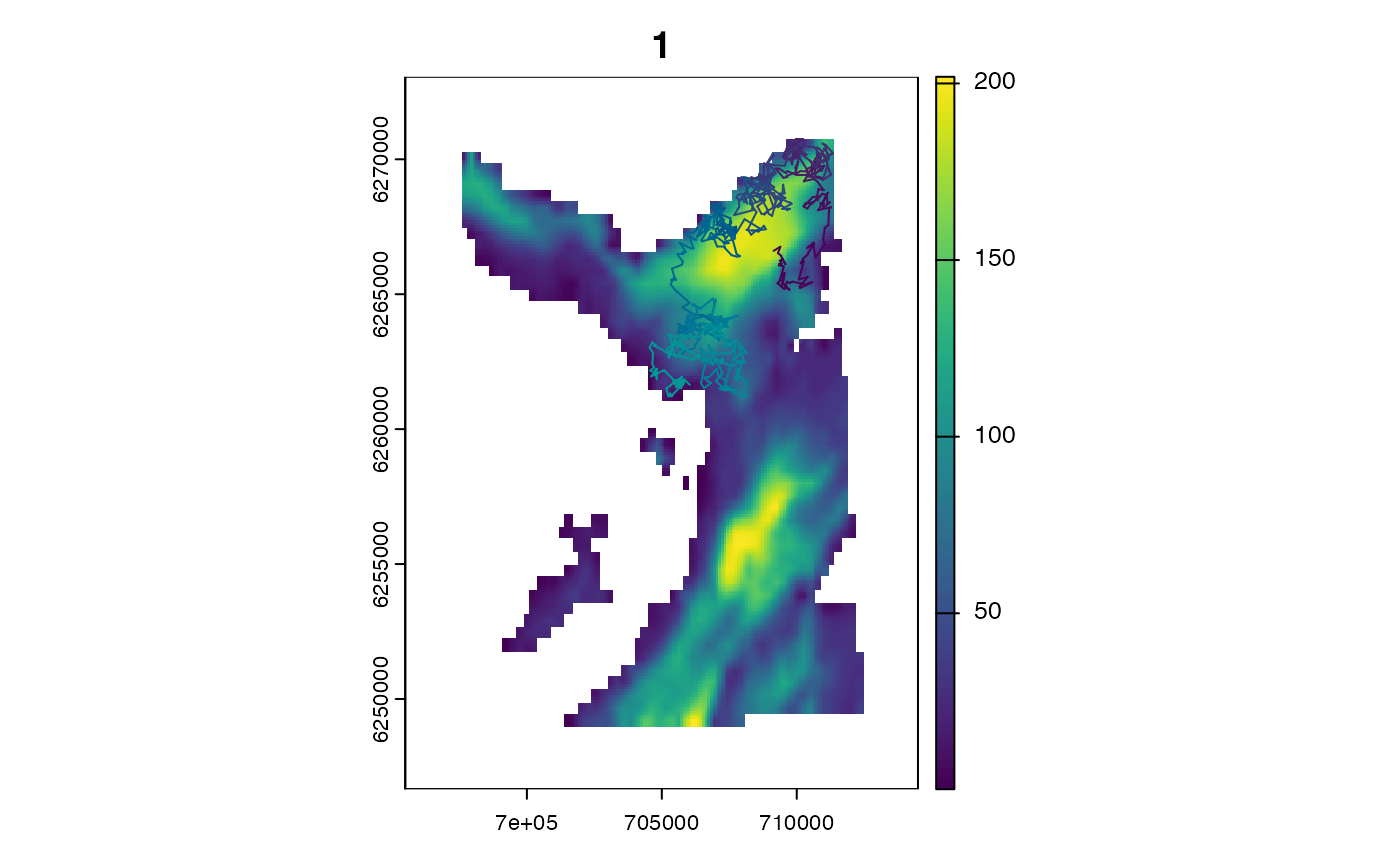
  #### Simulate path with default options
  paths <- sim_path_walk(.map = map,
                         .timeline = timeline,
                         .state = "StateXY",
                         .model_move = model_move_xy())

  #### Example (1): Simulate observations via `ModelObsAcousticLogisTrunc`

  # Overview:
  # * `ModelObsAcousticLogisTrunc`: observation model structure for acoustic observations
  # * See ?ModelObsAcousticLogisTrunc
  # * See JuliaCall::julia_help("ModelObs")
  # * This structure holds:
  #   - sensor_id (the receiver_id)
  #   - receiver_x, receiver_y (the receiver coordinates)
  #   - receiver_alpha, receiver_beta, receiver_gamma
  #   - (these are parameters of a truncated logistic detection probability model)
  # * Using these fields, it is possible to simulate detections at receivers

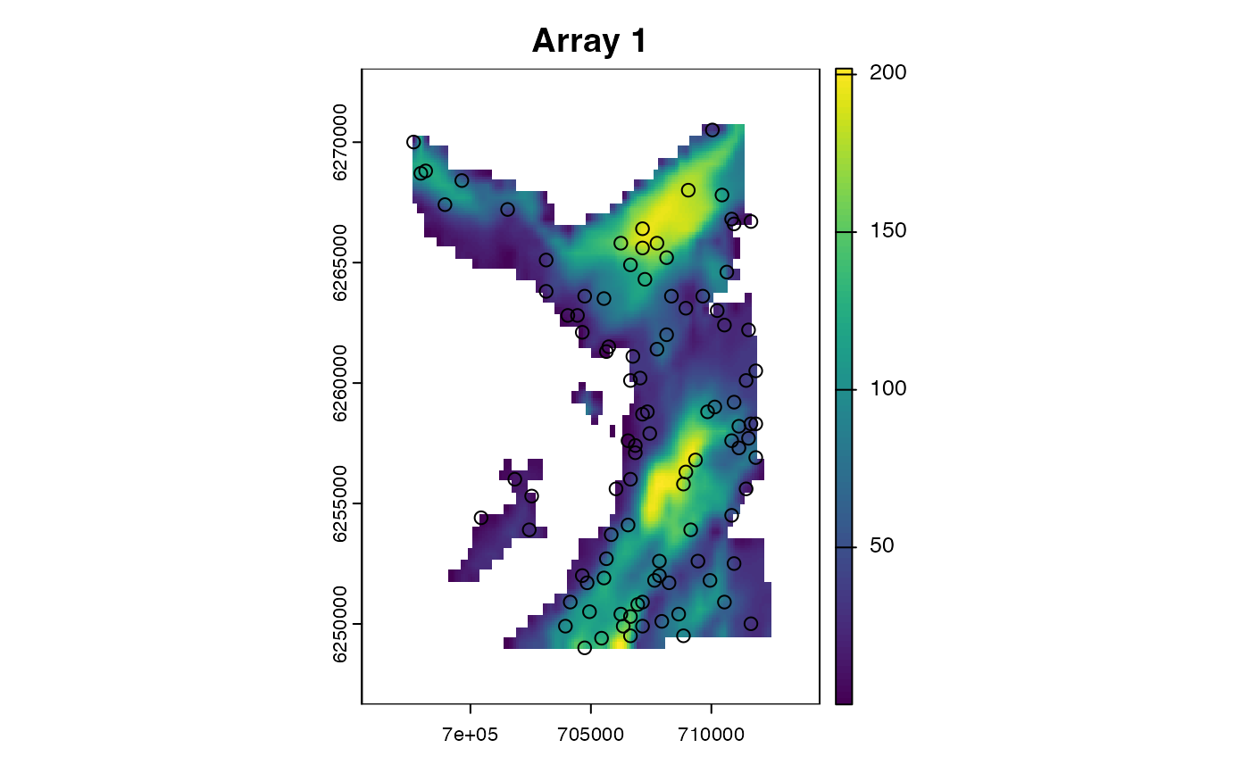
  # Simulate an acoustic array
  a <- 4
  b <- -0.01
  g <- 750
  moorings <- sim_array(.map = map,
                        .timeline = timeline,
                        .n_receiver = 100L,
                        # (optional) Define constant detection probability parameters
                        .receiver_alpha = a,
                        .receiver_beta = b,
                        .receiver_gamma = g)

  # This is the shape of detection probability model for the parameters we have chosen
  d <- seq(1, 1000, by = 1)
  plot(d, ifelse(d <= g, plogis(a * b * d), 0),
       ylab = "Detection probability",
       xlab = "Distance (m)",
       type = "l")

  # Define a data.table of observation model parameters
  moorings <-
    moorings |>
    select(sensor_id = "receiver_id",
           "receiver_x", "receiver_y",
           "receiver_alpha", "receiver_beta", "receiver_gamma") |>
    as.data.table()

  # Simulate observations
  obs <- sim_observations(.timeline = timeline,
                          .model_obs = list(ModelObsAcousticLogisTrunc = moorings))

  # Examine simulated observations
  # * sim_observations() returns a list, with one element for every `.model_obs`
  # * Each element is a `list`, with one element for each simulated path
  # * Each element is a [`data.table::data.table`] that contains the observations
  str(obs)

  # Plot detections
  detections <-
    obs$ModelObsAcousticLogisTrunc[[1]] |>
    lazy_dt() |>
    filter(obs == 1L) |>
    as.data.table()
  plot(detections$timestamp, detections$obs)

  # Customise `ModelObsAcousticLogisTrunc` parameters
  # > Receiver-specific parameters are permitted
  moorings[, receiver_alpha := runif(.N, 4, 5)]
  moorings[, receiver_beta := runif(.N, -0.01, -0.001)]
  moorings[, receiver_gamma := runif(.N, 500, 1000)]
  obs <- sim_observations(.timeline = timeline,
                          .model_obs = list(ModelObsAcousticLogisTrunc = moorings))

  #### Example (2): Simulate observations via `ModelObsDepthUniformSeabed`
  # `ModelObsDepthUniformSeabed` is an observation model for depth observations
  # * See ?ModelObsAcousticLogisTrunc
  # * See JuliaCall::julia_help("ModelObsAcousticLogisTrunc")
  pars <- data.frame(sensor_id = 1,
                     depth_shallow_eps = 10,
                     depth_deep_eps = 20)
  obs <- sim_observations(.timeline = timeline,
                          .model_obs = list(ModelObsDepthUniformSeabed = pars))

  #### Example (3): Simulate observations via `ModelObsDepthNormalTruncSeabed`
  # `ModelObsDepthNormalTruncSeabed` is an observation model for depth observations
  pars <- data.frame(sensor_id = 1,
                     depth_sigma = 10,
                     depth_deep_eps = 20)
  obs <- sim_observations(.timeline = timeline,
                          .model_obs = list(ModelObsDepthNormalTruncSeabed = pars))

  #### Example (4): Simulate observations via custom `ModelObs` sub-types
  # See `?ModelObs`

  #### Example (5): Use multiple observation models
  obs <- sim_observations(.timeline = timeline,
                          .model_obs = list(ModelObsAcousticLogisTrunc = moorings,
                                            ModelObsDepthNormalTruncSeabed = pars))
  str(obs)

}
#> `patter::julia_connect()` called @ 2025-04-22 09:32:18... 
#> ... Running `Julia` setup via `JuliaCall::julia_setup()`... 
#> ... Validating Julia installation... 
#> ... Setting up Julia project... 
#> ... Handling dependencies... 
#> ... `Julia` set up with 11 thread(s). 
#> `patter::julia_connect()` call ended @ 2025-04-22 09:32:18 (duration: ~0 sec(s)). 
#> Warning: Use `seq.POSIXt()` with `from`, `to` and `by` rather than `length.out` for faster handling of time stamps.



#> Warning: Use `seq.POSIXt()` with `from`, `to` and `by` rather than `length.out` for faster handling of time stamps.
#> List of 1
#>  $ ModelObsAcousticLogisTrunc:List of 1
#>   ..$ :Classes ‘data.table’ and 'data.frame':	100000 obs. of  8 variables:
#>   .. ..$ timestamp     : POSIXct[1:100000], format: "2016-01-01 00:00:00" "2016-01-01 00:00:00" ...
#>   .. ..$ obs           : int [1:100000] 0 0 0 0 0 0 0 0 0 0 ...
#>   .. ..$ sensor_id     : int [1:100000] 1 2 3 4 5 6 7 8 9 10 ...
#>   .. ..$ receiver_x    : num [1:100000] 709142 698042 708442 709942 701642 ...
#>   .. ..$ receiver_y    : num [1:100000] 6266607 6267507 6266307 6255107 6265107 ...
#>   .. ..$ receiver_alpha: num [1:100000] 4 4 4 4 4 4 4 4 4 4 ...
#>   .. ..$ receiver_beta : num [1:100000] -0.01 -0.01 -0.01 -0.01 -0.01 -0.01 -0.01 -0.01 -0.01 -0.01 ...
#>   .. ..$ receiver_gamma: num [1:100000] 750 750 750 750 750 750 750 750 750 750 ...
#>   .. ..- attr(*, ".internal.selfref")=<externalptr> 

#> Warning: Use `seq.POSIXt()` with `from`, `to` and `by` rather than `length.out` for faster handling of time stamps.
#> Warning: Use `seq.POSIXt()` with `from`, `to` and `by` rather than `length.out` for faster handling of time stamps.
#> Warning: Use `seq.POSIXt()` with `from`, `to` and `by` rather than `length.out` for faster handling of time stamps.
#> Warning: Use `seq.POSIXt()` with `from`, `to` and `by` rather than `length.out` for faster handling of time stamps.
#> List of 2
#>  $ ModelObsAcousticLogisTrunc    :List of 1
#>   ..$ :Classes ‘data.table’ and 'data.frame':	100000 obs. of  8 variables:
#>   .. ..$ timestamp     : POSIXct[1:100000], format: "2016-01-01 00:00:00" "2016-01-01 00:00:00" ...
#>   .. ..$ obs           : int [1:100000] 0 0 0 0 0 0 0 0 0 0 ...
#>   .. ..$ sensor_id     : int [1:100000] 1 2 3 4 5 6 7 8 9 10 ...
#>   .. ..$ receiver_x    : num [1:100000] 709142 698042 708442 709942 701642 ...
#>   .. ..$ receiver_y    : num [1:100000] 6266607 6267507 6266307 6255107 6265107 ...
#>   .. ..$ receiver_alpha: num [1:100000] 4.39 4.71 4.11 4.27 4.59 ...
#>   .. ..$ receiver_beta : num [1:100000] -0.00438 -0.0074 -0.0082 -0.00279 -0.00345 ...
#>   .. ..$ receiver_gamma: num [1:100000] 555 984 693 929 944 ...
#>   .. ..- attr(*, ".internal.selfref")=<externalptr> 
#>  $ ModelObsDepthNormalTruncSeabed:List of 1
#>   ..$ :Classes ‘data.table’ and 'data.frame':	1000 obs. of  5 variables:
#>   .. ..$ timestamp     : POSIXct[1:1000], format: "2016-01-01 00:00:00" "2016-01-01 00:02:00" ...
#>   .. ..$ obs           : num [1:1000] 40.2 34.9 41.9 58.5 41.3 ...
#>   .. ..$ sensor_id     : int [1:1000] 1 1 1 1 1 1 1 1 1 1 ...
#>   .. ..$ depth_sigma   : num [1:1000] 10 10 10 10 10 10 10 10 10 10 ...
#>   .. ..$ depth_deep_eps: num [1:1000] 20 20 20 20 20 20 20 20 20 20 ...
#>   .. ..- attr(*, ".internal.selfref")=<externalptr>