Plots: plot coordinates (x, y, t) — plot

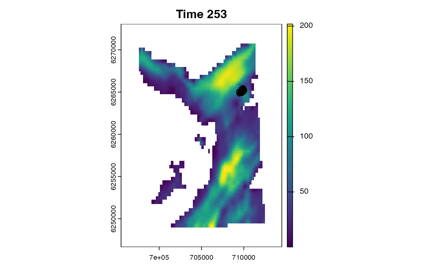
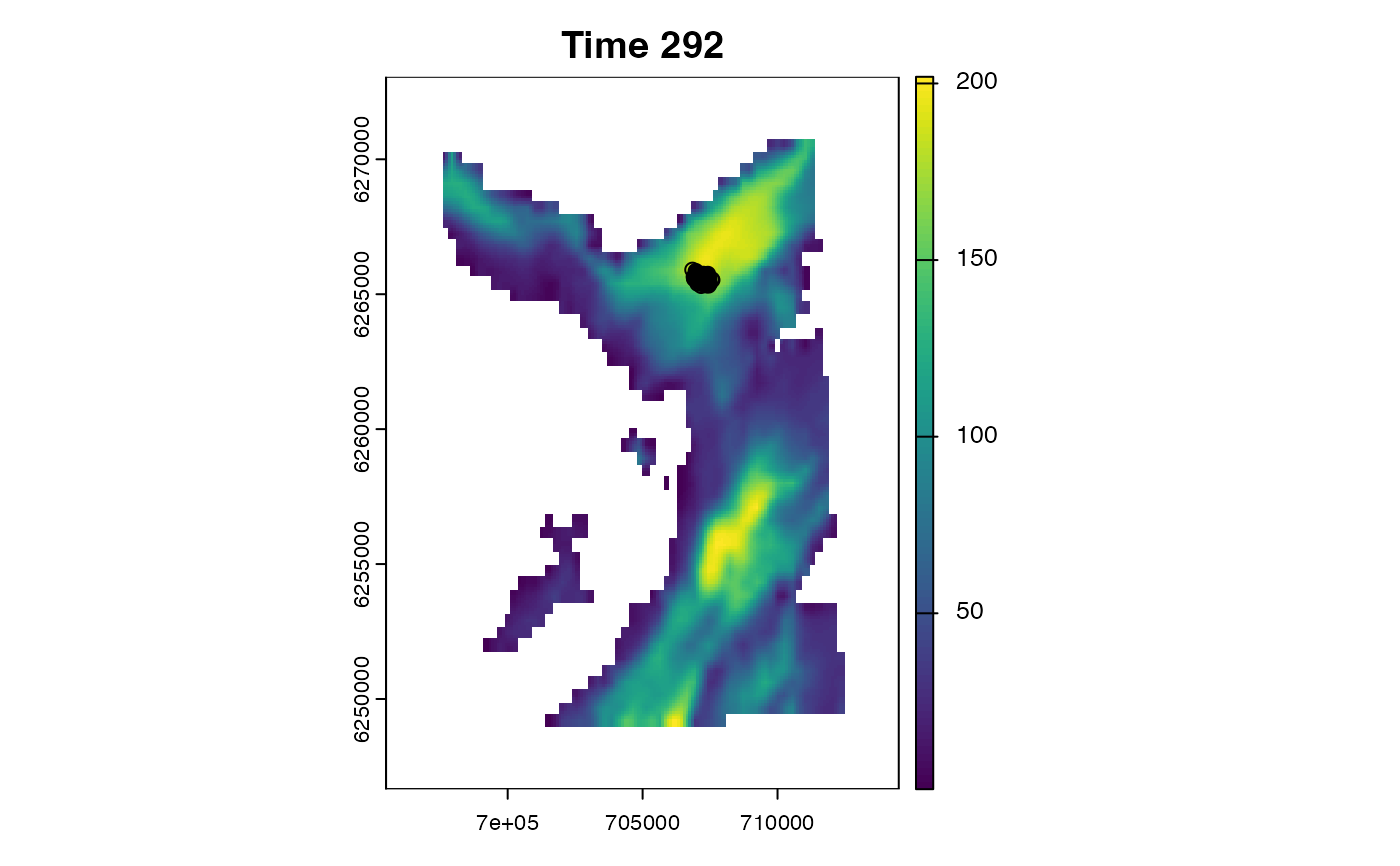
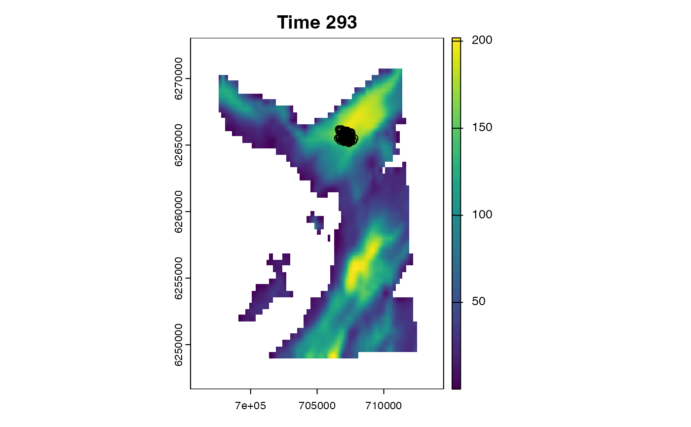
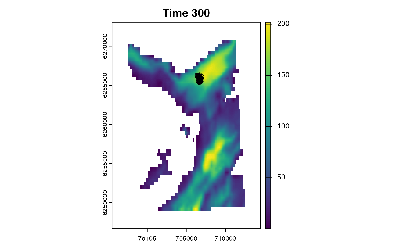
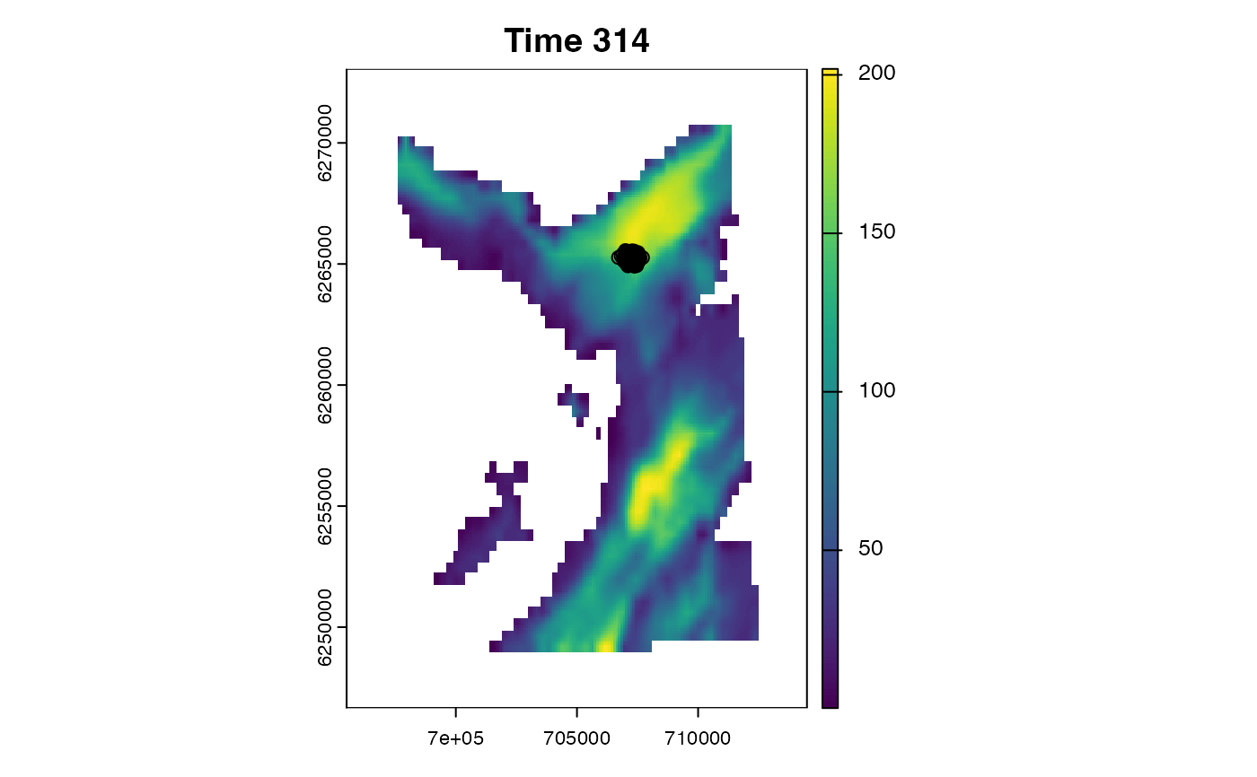
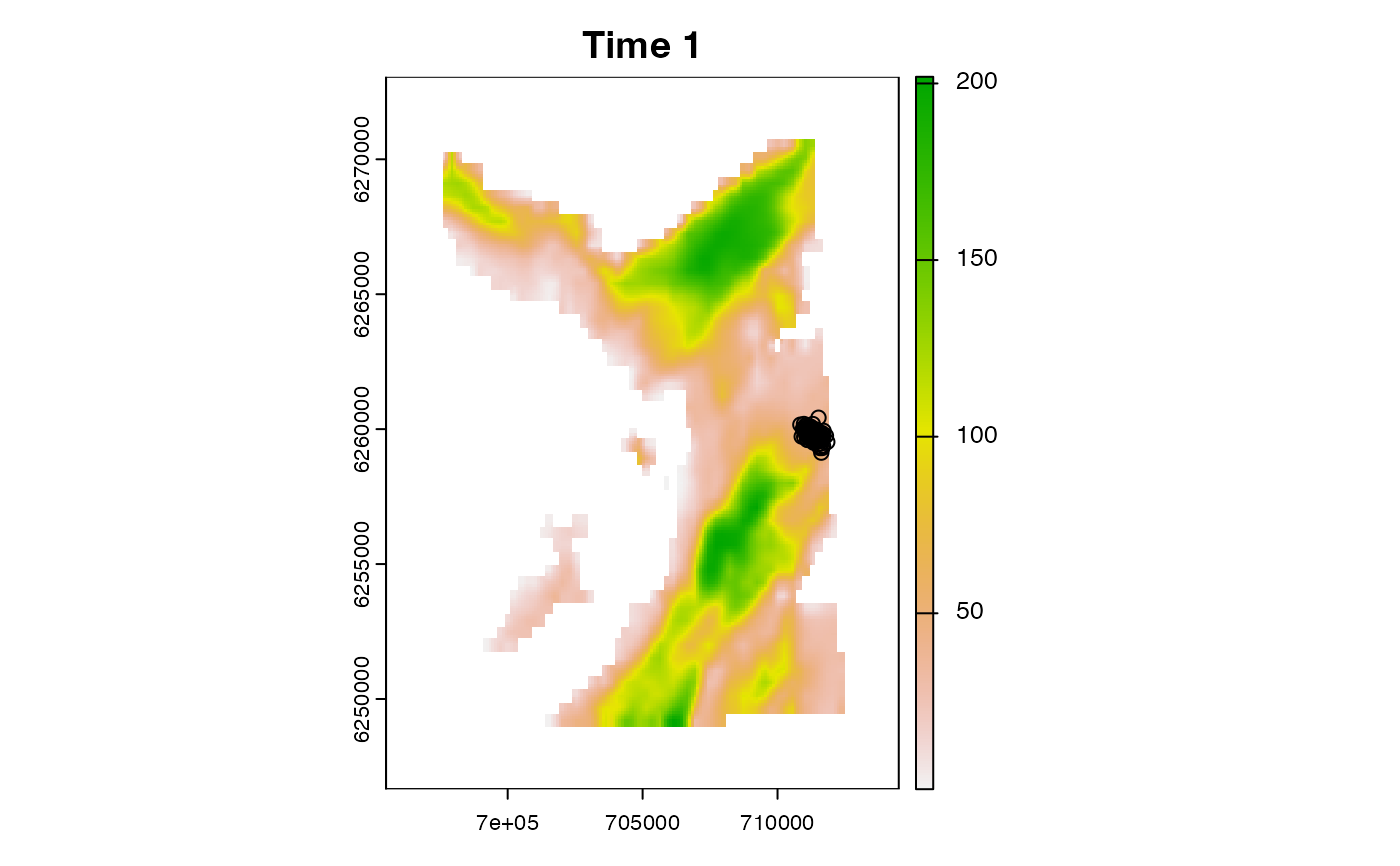
This function maps xyt data (i.e. coordinate (x, y) locations for selected time steps (t) or entire time series) and can be used to create animations.

Usage

plot_xyt(
  .map,
  .coord,
  .steps = NULL,
  .png = NULL,
  .add_surface = list(),
  .add_points = list(),
  .add_layer = NULL,
  .prompt = FALSE,
  ...
)

Arguments

.map

A terra::SpatRaster that defines the study area (see glossary).

.coord

A data.table::data.table of coordinates, including x, y and timestep columns. Point graphical parameters (pch, col, bg, cex, lwd, lty, lwd) can be included as columns to customise point appearance. (Graphical parameters provided here silently overwrite any elements of the same name in .add_points.)

.steps

NULL or an integer vector of the time steps for which to map coordinates (e.g., .steps = 1:5L). NULL specifies all time steps.

.png

(optional) A named list, passed to grDevices::png(), to save plots to file. filename should be the directory in which to write files. Files are named {.steps[1]}.png, {.steps[2]}.png, ..., {.steps[N]}.png. .png should be supplied if .cl is supplied via ....

.add_surface, .add_points

Named lists for plot customisation.

.add_surface is passed to terra::plot(), excluding x and main.
.add_points is passed to graphics::points(), excluding x and y.

.add_layer

(optional) A function used to add additional layer(s) to the plot. The function must a single (unnamed) integer value for the time step (even if ignored). An example function is function(...) points(x, y) where x and y are (for example) receiver coordinates.

.prompt

A logical variable that defines whether or not to prompt the user for input between plots. This is only used in interactive mode if .png = NULL (and there are multiple time steps).

...

Additional argument(s) passed to cl_lapply(), such as .cl.

Value

The function is called for its side effects. It returns invisible(TRUE).

Details

For each .step, terra::plot() is used to plot .map. Coordinates in .coord are added onto the grid via graphics::points(). (Note that coordinates derived from particle algorithms are equally weighted thanks to resampling.)

This function replaces flapper::pf_plot_history().

On Linux, this function cannot be used within a Julia session.

Author

Edward Lavender

Examples

if (patter_run(.julia = FALSE, .geospatial = TRUE)) {

  #### Set up
  # Define map
  map <- dat_gebco()
  # Define particle samples
  fwd <- dat_pff()$states
  bwd <- dat_pfb()$states
  smo <- dat_tff()$states
  # Define directories
  con    <- file.path(tempdir(), "patter")
  frames <- file.path(con, "frame")
  mp4s   <- file.path(con, "mp4")
  dir.create(frames, recursive = TRUE)
  dir.create(mp4s, recursive = TRUE)
  # Cluster options
  pbo <- pbapply::pboptions(nout = 4L)

  #### Example (1): Plot selected samples
  # Plot particles from the forward filter
  plot_xyt(.map = map,
             .coord = fwd,
             .steps = 1L)
  # Plot particles from the backward filter
  plot_xyt(.map = map,
             .coord = bwd,
             .steps = 1L)
  # Plot smoothed particles
  plot_xyt(.map = map,
             .coord = smo,
             .steps = 1L)

  #### Example (2): Plot multiple time steps
  # Specify selected steps
  plot_xyt(.map = map,
             .coord = smo,
             .steps = 1:4L)
  # Plot all steps (default: .step = NULL)
  plot_xyt(.map = map,
             .coord = fwd)
  # Use `.prompt = TRUE`
  plot_xyt(.map = map,
             .coord = smo,
             .steps = 1:4L,
             .prompt = TRUE)

  #### Example (3): Customise the background map via `.add_surface`
  plot_xyt(.map = map,
             .coord = smo,
             .steps = 1L,
             .add_surface = list(col = rev(terrain.colors(256L))))

  #### Example (4): Customise the points
  # Use `.add_points`
  plot_xyt(.map = map,
             .coord = smo,
             .steps = 1L,
             .add_points = list(pch = ".", col = "red"))
  # Include `points()` arguments as columns in `.coord`
  # * Here, we colour branches from the filter pruned by the smoother in red
  fwd[, cell_id := terra::extract(map, cbind(x, y))]
  bwd[, cell_id := terra::extract(map, cbind(x, y))]
  smo[, cell_id := terra::extract(map, cbind(x, y))]
  fwd[, col := ifelse(cell_id %in% smo$cell_id, "black", "red")]
  bwd[, col := ifelse(cell_id %in% smo$cell_id, "black", "red")]
  plot_xyt(.map = map,
             .coord = rbind(fwd, bwd),
             .steps = 1L,
             .add_points = list(pch = "."))

  #### Example (5): Add additional map layers
  plot_xyt(.map = map,
             .coord = smo,
             .steps = 1L,
             .add_layer = function(t) mtext(side = 4, "Depth (m)", line = -4))

  #### Example (6): Write images to file
  # Write images in serial
  plot_xyt(.map = map,
             .coord = smo,
             .steps = 1:4L,
             .png = list(filename = frames))
  # Use a fork cluster
  if (.Platform$OS.type == "unix") {
    plot_xyt(.map = map,
               .coord = smo,
               .steps = 1:4L,
               .png = list(filename = frames),
               .cl = 2L,
               .chunk = TRUE)
  }

  #### Example (7): Make animations
  if (rlang::is_installed("av")) {

    # There are lots of tools to create animations:
    # * `av::av_encode_video()`       # uses ffmpeg
    # * `animation::saveVideo()`      # uses ffmpeg
    # * `magick::image_write_video()` # wraps av()
    # * `glatos::make_video()`        # wraps av()

    # Helper function to open (mp4) files
    Sys.open <- function(.file) {
      if (.Platform$OS.type == "Windows") {
        cmd <- paste("start", shQuote(.file))
      } else {
        cmd <- paste("open", shQuote(.file))
      }
      system(cmd)
    }

    # Use av::av_encode_video()
    # * This is one of the faster options
    input   <- file_list(frames)
    output  <- file.path(mp4s, "ani.mp4")
    av::av_encode_video(input, output, framerate = 10)
    # Sys.open(output)

  }

  file_cleanup(con)

}





















































































































































































































































































































































































#> `cl_lapply()` implemented on 2 core(s) using a total of 4 chunk(s) (~2 per core & progress gradations).

Plots: plot coordinates (`x`, `y`, `t`)