Movement model plots

plot() methods for movement models (see ModelMove).

Usage

# S3 method for class 'ModelMoveXY'
plot(x, .panel_length = list(), .panel_heading = list(), .par = list(), ...)

# S3 method for class 'ModelMoveXYZ'
plot(
  x,
  .panel_length = list(),
  .panel_heading = list(),
  .panel_z = list(),
  .par = list(),
  ...
)

# S3 method for class 'ModelMoveCXY'
plot(
  x,
  .panel_length = list(),
  .panel_heading_delta = list(),
  .par = list(),
  ...
)

# S3 method for class 'ModelMoveCXYZ'
plot(
  x,
  .panel_length = list(),
  .panel_heading_delta = list(),
  .panel_z_delta = list(),
  .par = list(),
  ...
)

Arguments

x

A ModelMove-class object from a model_move_*() function (e.g., model_move_xy().

.panel_length, .panel_heading, .panel_heading_delta, .panel_z, .panel_z_delta

Panel properties:

NULL suppresses the panel;
list() uses default graphical arguments;
A named list of arguments, passed to plot(), customises the panel;

.par

Graphical parameters:

NULL uses current graphical parameters;
list() uses default graphical parameters;
A named list of arguments, passed to par(), customises parameters;

...

Additional arguments, passed to plot(), which affect all panels;

Value

The functions produce a plot. invisible(NULL) is returned.

Details

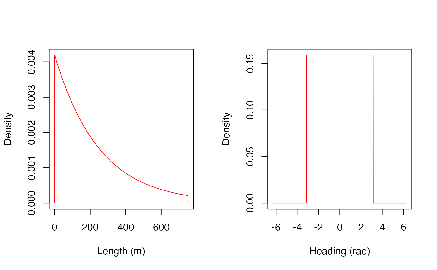
For each in-built ModelMove-class (e.g., ModelMoveXY), a corresponding plot() method is provided that plots the component probability-density distributions (e.g., the distribution of step lengths and turning angles) for any model instance. Under default options, a multi-panelled plot is produced, with one panel for each model dimension (e.g., the step length and the heading). Use .panel_* arguments to customise individual panels, .par to set graphical parameters and ... to customise all panels. Set .panel_* xlim to specify the x-axis range over which distributions are shown. If unspecified, probability density is plotted along a predefined range or from the 0.0001 to 0.9999 quantiles of the distribution.

Author

Edward Lavender

Examples

if (patter_run(.julia = TRUE, .geospatial = FALSE)) {

  julia <- julia_connect()
  map <- dat_gebco(.return = "character")
  set_map(map)

  #### Example (1): Plot movement models
  # Plot default models
  plot(model_move_xy())
  plot(model_move_xyz())
  plot(model_move_cxy())
  plot(model_move_cxyz())
  # Plot customised model
  plot(model_move_cxyz(.dbn_length = "truncated(Normal(0.0, 100.0),
                                        lower = 0.0, upper = 1000.0)"))

  #### Example (2): Use `...` to pass graphical arguments to all panels
  plot(model_move_xy(), col = "red")

  #### Example (3): Use `.panel_* = NULL` to suppress selected panels
  plot(model_move_xy(),
       .panel_heading = NULL)

  #### Example (4): Customise individual panels via `.panel_*` lists
  plot(model_move_xy(),
       .panel_length = list(main = "A"),
       .panel_heading = list(main = "B"))

  #### Example (5): Control graphical parameters via the `.par` list
  # Use default options
  plot(model_move_xy(), .par = list())
  # Specify par options
  plot(model_move_xy(), .par = list(oma = c(3, 3, 3, 3)))
  # Set `.par = NULL` to leave `par` unchanged
  pp <- par(mfrow = c(2, 1))
  plot(model_move_xy(), .par = NULL)
  par(pp)

  #### Example (6): Simulate reasliations of the movement model
  # See `?sim_path_walk()`
  # Set `.map` argument to visualise trajectories
  # (On Linux, this is only possible if JULIA_SESSION = "FALSE")
  sim_path_walk(.timeline = seq(as.POSIXct("2016-01-01", tz = "UTC"),
                                as.POSIXct("2016-01-01 12:00:00", tz = "UTC"),
                                by = "2 mins"),
                .state = "StateXY",
                .model_move = model_move_xy())

}
#> `patter::julia_connect()` called @ 2025-04-22 09:31:48... 
#> ... Running `Julia` setup via `JuliaCall::julia_setup()`... 
#> ... Validating Julia installation... 
#> ... Setting up Julia project... 
#> ... Handling dependencies... 
#> ... `Julia` set up with 11 thread(s). 
#> `patter::julia_connect()` call ended @ 2025-04-22 09:31:48 (duration: ~0 sec(s)). 











#>      path_id timestep           timestamp map_value        x       y
#>        <int>    <int>              <POSc>     <num>    <num>   <num>
#>   1:       1        1 2016-01-01 00:00:00  89.09113 705642.1 6264507
#>   2:       1        2 2016-01-01 00:02:00 105.07728 705973.6 6264847
#>   3:       1        3 2016-01-01 00:04:00 105.07728 705977.2 6264825
#>   4:       1        4 2016-01-01 00:06:00 150.48004 706228.4 6265426
#>   5:       1        5 2016-01-01 00:08:00 132.10489 706243.0 6265074
#>  ---                                                                
#> 357:       1      357 2016-01-01 11:52:00  86.40712 710335.2 6266947
#> 358:       1      358 2016-01-01 11:54:00  97.41836 710385.0 6266960
#> 359:       1      359 2016-01-01 11:56:00 135.54185 710210.1 6267495
#> 360:       1      360 2016-01-01 11:58:00 117.44244 710399.4 6267577
#> 361:       1      361 2016-01-01 12:00:00 144.81311 710093.4 6267510