Pretty two-dimensional predictions — pretty_predictions

This is function plots pretty two-dimensional predictions from a statistical model.

pretty_predictions_2d(
  x,
  view = NULL,
  n_grid = 30,
  cond = list(),
  predict_param = list(),
  select = "fit",
  xlim = NULL,
  ylim = NULL,
  zlim = NULL,
  xlab = NULL,
  ylab = NULL,
  pretty_axis_args = list(side = 1:4, axis = list(list(), list(), list(labels = FALSE),
    list(labels = FALSE))),
  col_pal = viridis::viridis,
  col_n = 100,
  add_xy = NULL,
  add_rug_x = NULL,
  add_rug_y = NULL,
  add_contour = NULL,
  add_legend = NULL,
  legend_breaks = NULL,
  legend_labels = NULL,
  legend_x = NULL,
  legend_y = NULL,
  ...
)

Arguments

x	A model (e.g. an output from `gam`).
view	A character vector of two variables that define the variables on the x and y axis.
n_grid, cond, predict_param, select	Prediction controls. `n_grid` is an integer that defines the resolution of the surface (in both x and y directions). `cond` (optional) is a named list that defines the values of other predictors (i.e., those not in `view`) for which to make predictions. If un-supplied, factor variables are set at the most commonly occuring factor level and continuous variables are set at the closest observed value to the median. `predict_param` (optional) A named list of arguments, passed to `predict`, to customise predictions. `select` (optional) If the call to `predict` returns a list, `select` is the name of the element in that list that is plotted (e.g., `"fit"` or `"se.fit"`). If the call to `predict` returns a numeric vector, this is ignored.
xlim, ylim, zlim	Axis limits.
xlab, ylab	X and y axis labels.
pretty_axis_args	A named list of arguments, passed to `pretty_axis`, to control axes.
col_pal, col_n	Colour controls. `col_pal` is a colour palette function from which colours are drawn. `col_n` is the number of colours to use in the colour scheme.
add_xy	A named list of arguments, passed to `points`, to add observations to the plot. `add_xy = NULL` suppresses this option, `add_xy = list()` implements default arguments and a named list customises these.
add_rug_x, add_rug_y	Named list of arguments, passed to `rug`, to add observed values of the variables defined in `view` to the plot. `add_rug_* = NULL` suppresses this option, `add_rug_*` implements default arguments and a named list customises these.
add_contour	A named list of arguments, passed to `contour`, to add contour lines to the plot. `add_contour = NULL` suppresses this option, `add_contour = list()` implements default arguments and a named list customises these.
add_legend, legend_breaks, legend_labels, legend_x, legend_y	Legend controls. `add_legend` A named list of arguments, passed to `add_colour_bar`, to add a legend to the plot. `add_legend = NULL` suppresses this option, `add_legend = list()` implements default arguments and a named list customises these. `legend_breaks` and `legend_labels` are functions that modify the legend breaks and legend labels respectively. `legend_x` and `legend_y` are numeric vectors of length two that specify the x and y positions, on the current plot, for the four corners of the legend. If un-supplied, the two `legend_x` coordinates are taken as the maximum x limit of x plus (a) 1 per cent and (b) 10 per cent of the difference between the maximum and minimum x limits. `legend_y` is taken from `ylim`.
...	Additional arguments passed to `image`, which is used for plotting (excluding `col`, `breaks` and `axes` which are defined internally).

Value

The function returns a contour plot of the predictions of a model for the two variables defined in view and, invisibly, a named list containing the prediction matrix (`z') and the list of pretty axis parameters produced by pretty_axis (`axis_ls').

Details

This function was motivated by vis.gam (see also pretty_smooth_2d).

Author

Edward Lavender

Examples

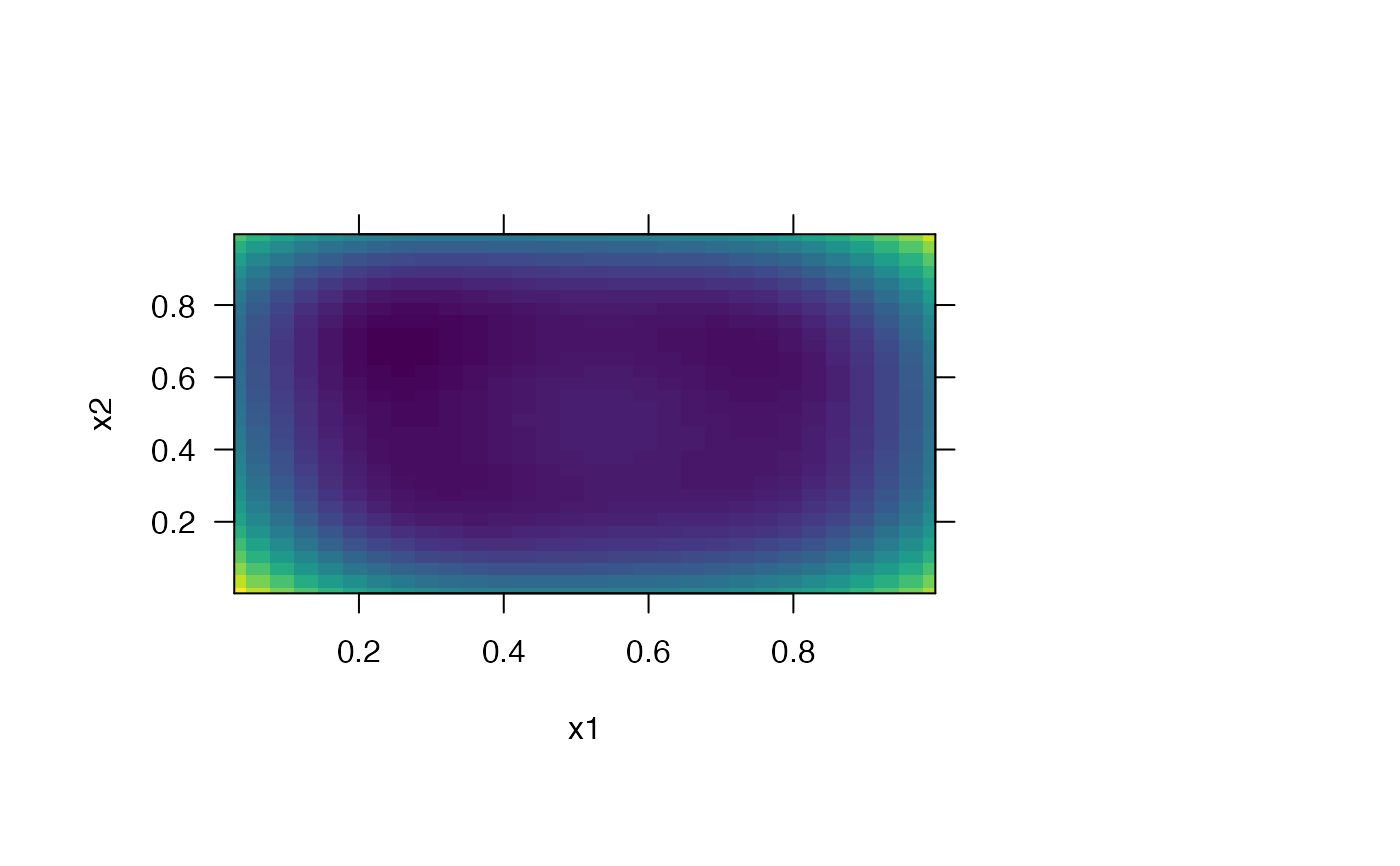
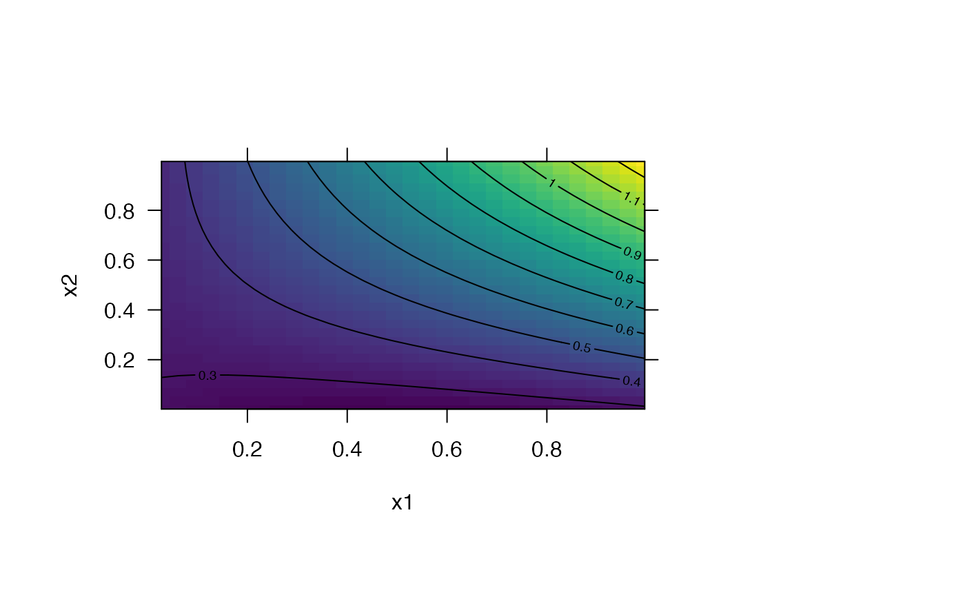
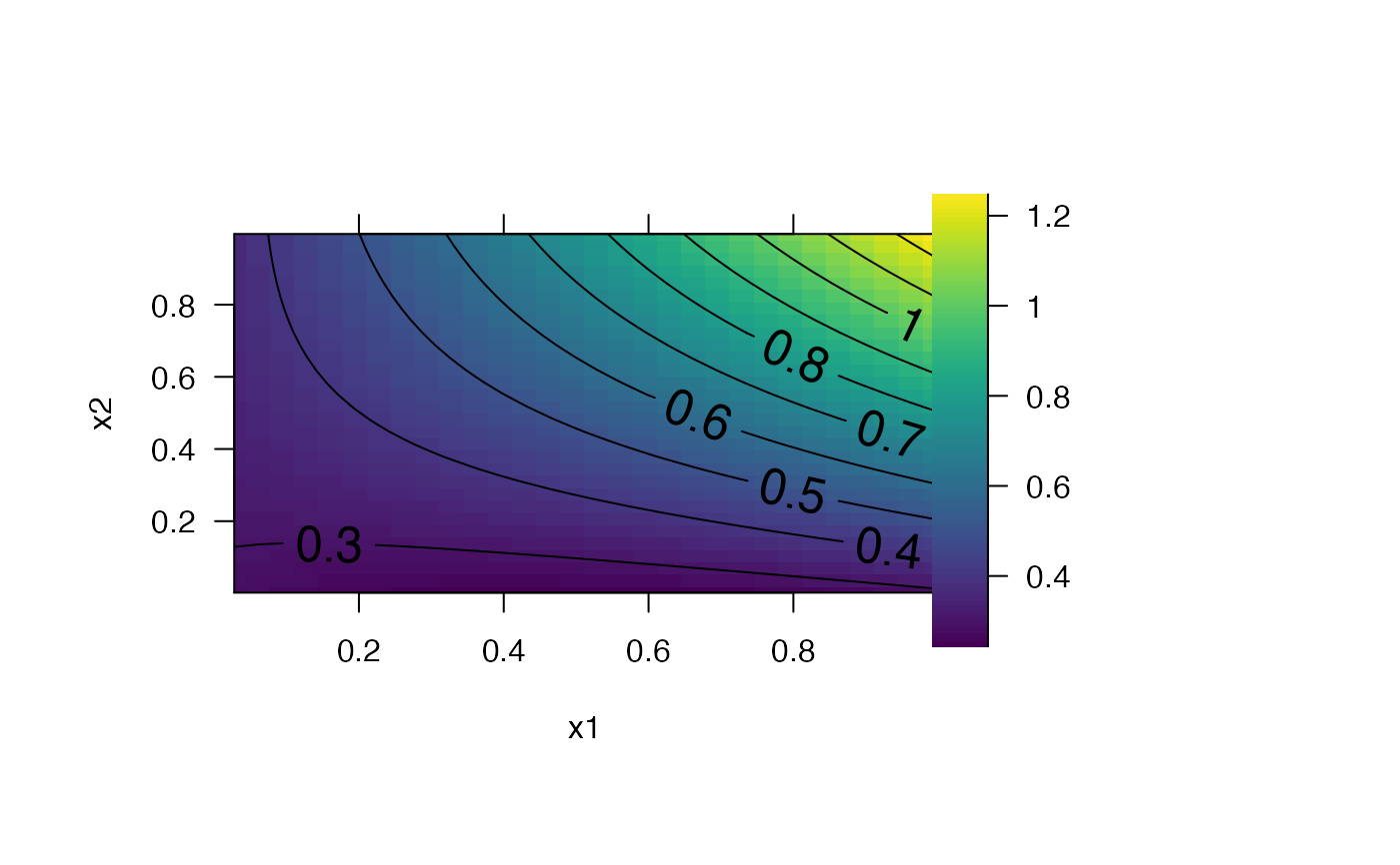
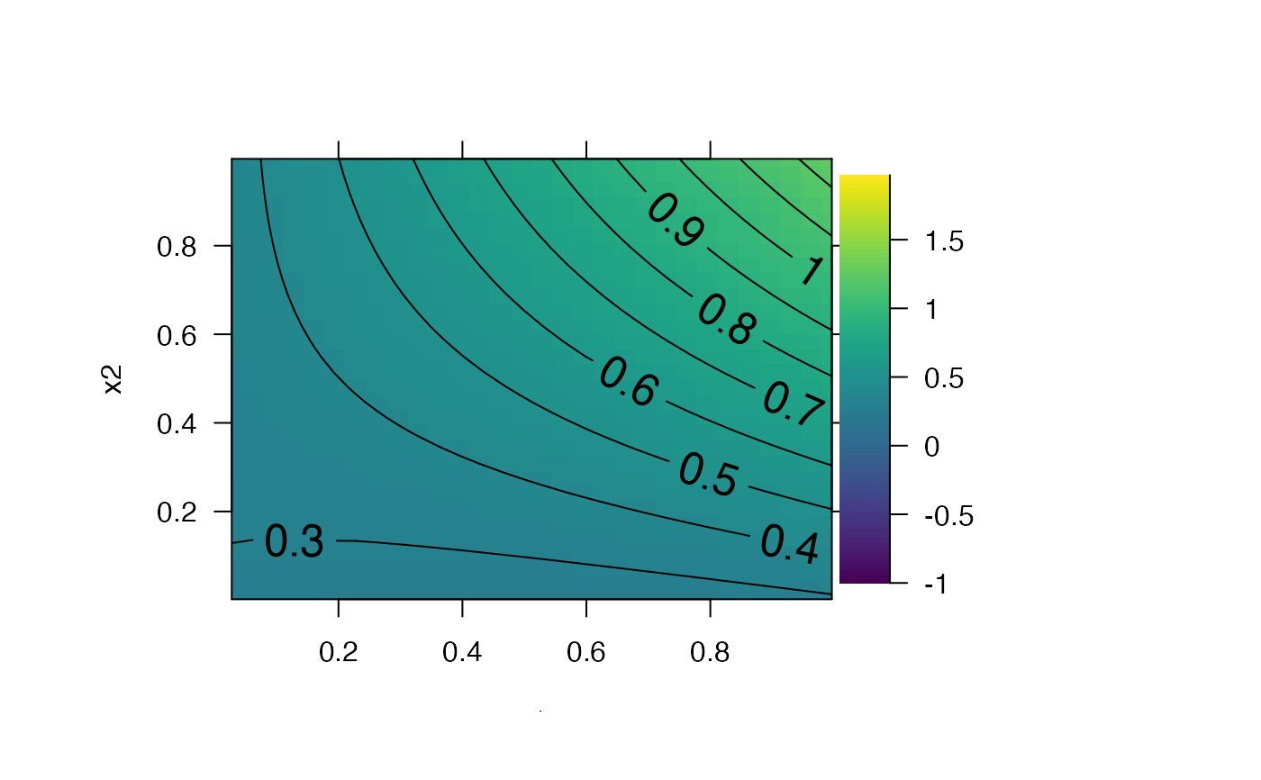
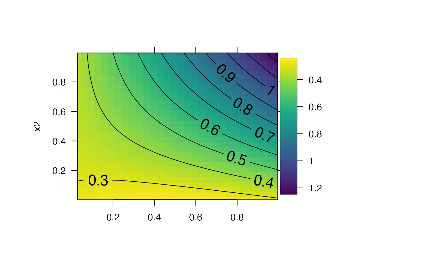
#### Simulate example data and fit model (following ?mgcv::vis.gam examples)
set.seed(0)
n    <- 200
sig2 <- 4
x0   <- runif(n, 0, 1)
x1   <- runif(n, 0, 1)
x2   <- runif(n, 0, 1)
y    <- x0^2 + x1 * x2 + runif(n, -0.3, 0.3)
g    <- mgcv::gam(y ~ s(x0, x1, x2))

#### Example (1): Contour plot using default options
pp <- par(oma = c(2, 2, 2, 10))
pretty_predictions_2d(g, view = c("x1", "x2"))

#### Example (2): Customise predictions
# Use n_grid to control the grid resolution
pretty_predictions_2d(g, view = c("x1", "x2"), n_grid = 10)
# Use cond to set other variables at specific values
pretty_predictions_2d(g, view = c("x1", "x2"), cond = list(x0 = mean(x0)))
# Use predict_param for further control, e.g., to plot SEs
pretty_predictions_2d(g, view = c("x1", "x2"),
                      predict_param = list(se.fit = TRUE), select = "se.fit")

#### Example (3): Customise colours
# Use col_pal and col_n
pretty_predictions_2d(g, view = c("x1", "x2"),
                      col_pal = grDevices::heat.colors,
                      col_n = 10)
pretty_predictions_2d(g, view = c("x1", "x2"),
                      col_pal = grDevices::heat.colors,
                      col_n = 100)

#### Example (4): Customise axes via xlim, ylim and pretty_axis_args
# Use xlim and ylim
pretty_predictions_2d(g, view = c("x1", "x2"),
                      xlim = c(0, 1),
                      ylim = c(0, 1))
# Use pretty_axis_args
pretty_predictions_2d(g, view = c("x1", "x2"),
                      pretty_axis_args = list(side = 1:4))

#### Example (5): Add observed data
# Specify list() to use default options
pretty_predictions_2d(g, view = c("x1", "x2"),
                      add_xy = list())
# Customise addition of observed data
pretty_predictions_2d(g, view = c("x1", "x2"),
                      add_xy = list(pch = ".'", cex = 5))

#### Example (6): Add rugs for the x and y variables
# Use default options
pretty_predictions_2d(g, view = c("x1", "x2"),
                      add_rug_x = list(),
                      add_rug_y = list())
# Customise options
pretty_predictions_2d(g, view = c("x1", "x2"),
                      add_rug_x = list(col = "grey"),
                      add_rug_y = list(col = "grey"))

#### Example (7): Add contours
# Use default options
pretty_predictions_2d(g, view = c("x1", "x2"),
                      add_contour = list())
# Customise contours
pretty_predictions_2d(g, view = c("x1", "x2"),
                      add_contour = list(labcex = 1.5))

#### Example (8): Add add_colour_bar()
# Use default options
pp <- graphics::par(oma = c(2, 2, 2, 10))
pretty_predictions_2d(g,
                      view = c("x1", "x2"),
                      add_contour = list(labcex = 1.5),
                      add_legend = list())
graphics::par(pp)
# Customise colour bar
pp <- graphics::par(oma = c(2, 2, 2, 10))
pretty_predictions_2d(g,
                      view = c("x1", "x2"),
                      add_contour = list(labcex = 1.5),
                      zlim = c(-1, 2), add_legend = list())
graphics::par(pp)
# E.g., reverse the colour scheme and legend
# ... This is useful if, for example, the surface represents the depth of an
# ... animal, in which case it is natural to have shallower depths near the
# ... top of the legend.
pp <- graphics::par(oma = c(2, 2, 2, 10))
pretty_predictions_2d(g, view = c("x1", "x2"),
                      col_pal = function(n) rev(viridis::viridis(n)),
                      add_contour = list(labcex = 1.5),
                      add_legend = list(),
                      legend_breaks = function(x) x *-1,
                      legend_labels = abs)
graphics::par(pp)